Case Based Reasoning: Teaching AI to Learn From itself

✨ Summary
Imagine an AI that gets smarter every time it works not by retraining on massive datasets, but by learning from its own reasoning and reflection, just like humans.
Most AI systems are frozen in time. Trained once, deployed forever, they never learn from mistakes or build on successes. Real intelligence human or artificial doesn’t work that way. It learns from experience.
This is the vision behind Stephanie: a self-improving AI that gets better every time it acts, not by fine-tuning, but by remembering, reusing, and revising its reasoning.
In this post, we implement the core ideas of the Memento: Fine-tuning LLM Agents without Fine-tuning LLMs paper inside Stephanie.
By the end, you’ll see how case-based reasoning, multi-dimensional scoring, and retention policies combine to give Stephanie something most AI systems lack: the ability to truly learn from experience.
🧐 Hierarchical Reasoning Model (HRM)
👉 See Post: Layers of thought: smarter reasoning with the Hierarchical Reasoning Model
Before we can teach Stephanie to reuse her reasoning, we first need a way to judge its quality.
The paper HRM: Hierarchical Reasoning Model introduced a new way to think. The Hierarchical Reasoning Model (HRM) gives Stephanie the ability to reason in layers. Instead of jumping straight from input to output, HRM breaks problems down into:
- High-level strategy (HModule) 🧭 – setting the overall plan.
- Low-level analysis (LModule) 🔍 – working through details step by step.
- Nested loops 🔄 – iterating between the two, refining judgment until confident.
This matters because self-improvement requires reflection. Other scorers (MRQ, SICQL, EBT, SVM) give useful numbers, but HRM provides a reasoned judgment with a trace of how it got there essential for Case-Based Reasoning and middleware reuse.
🎨 Simplified Flow of HRM
    flowchart LR
    A["📄 Input (Goal + Doc)"]:::data --> B["🎯 Input Projector"]:::module
    B --> C["🧭 HModule<br/>High-Level Strategy"]:::module
    C --> D["🔍 LModule<br/>Detail Analysis"]:::module
    D --> E["🔄 Nested Loop<br/>(N cycles × T steps)"]:::loop
    E --> C
    C --> F["📊 Final Output<br/>Reasoned Score"]:::data

    classDef data fill:#e8f5e9,stroke:#2e7d32,stroke-width:2px;
    classDef module fill:#e3f2fd,stroke:#1565c0,stroke-width:2px;
    classDef loop fill:#fff3e0,stroke:#ef6c00,stroke-width:2px;
This diagram is deliberately simplified: one input ➝ strategy ➝ details ➝ loop ➝ final judgment. It emphasizes why HRM is different it thinks before it answers.
🏗️ Building HRM in Code
Now that we’ve seen why HRM matters and how it works conceptually, let’s translate that into code. The implementation is deliberately modular:
- RMSNorm ⚖️ keeps reasoning stable across long loops.
- RecurrentBlock 🔄 powers both the detail-focused LModule and the strategy-focused HModule.
- InputProjector 🎯 prepares raw embeddings for reasoning.
- OutputProjector 📊 transforms the final high-level state into a usable score.
- HRMModel 🧠 ties it all together into a nested loop that alternates between fine-grained updates and high-level adjustments.
What follows is the full PyTorch definition of the HRM. It’s designed to mirror the reasoning loop we discussed earlier low-level analysis inside high level cycles, converging toward a reasoned judgment rather than a one-shot score.
import torch
import torch.nn as nn

class RMSNorm(nn.Module):
    """
    Root Mean Square Normalization (RMSNorm).
    Unlike LayerNorm, it normalizes across features without subtracting the mean.
    This keeps scale consistent while letting the network learn its own balance.
    """
    def __init__(self, dim: int, eps: float = 1e-6):
        super().__init__()
        self.eps = eps
        # Each feature gets a learned scaling weight
        self.weight = nn.Parameter(torch.ones(dim))

    def _norm(self, x):
        # Normalize by root mean square (RMS) of activations
        return x * torch.rsqrt(x.pow(2).mean(-1, keepdim=True) + self.eps)

    def forward(self, x):
        output = self._norm(x.float()).type_as(x)
        return output * self.weight


class RecurrentBlock(nn.Module):
    """
    Recurrent update block used in both HRM modules:
      - LModule (low-level thinker)
      - HModule (high-level planner)

    Internally: GRUCell + RMSNorm
    - GRUCell gives temporal memory (keeps track of past reasoning)
    - RMSNorm stabilizes hidden state scale
    """
    def __init__(self, input_dim, hidden_dim, name="RecurrentBlock"):
        super().__init__()
        self.name = name
        self.rnn_cell = nn.GRUCell(input_dim, hidden_dim)
        self.norm = RMSNorm(hidden_dim)

    def forward(self, z_prev, input_combined):
        """
        One reasoning update step.
        - z_prev: previous hidden state (B, hidden_dim)
        - input_combined: current inputs (B, input_dim)
        Returns: next hidden state (B, hidden_dim)
        """
        z_next = self.rnn_cell(input_combined, z_prev)
        z_next = self.norm(z_next)  # keep scale in check
        return z_next

    def init_state(self, batch_size, hidden_dim, device):
        """Start with zero-initialized memory."""
        return torch.zeros(batch_size, hidden_dim, device=device)


class InputProjector(nn.Module):
    """
    Projects the raw input embedding into HRM's reasoning space.
    This is the 'x_tilde' vector   the problem seen through Stephanie's
    cognitive lens before reasoning begins.
    """
    def __init__(self, input_dim, hidden_dim):
        super().__init__()
        self.project = nn.Linear(input_dim, hidden_dim)
        self.norm = RMSNorm(hidden_dim)

    def forward(self, x):
        x_proj = self.project(x)
        x_tilde = self.norm(x_proj)
        return x_tilde


class OutputProjector(nn.Module):
    """
    Projects the final high-level hidden state (zH) to the output space.
    In HRM this is usually a scalar quality score (e.g., epistemic value).
    """
    def __init__(self, h_dim, output_dim):
        super().__init__()
        self.project = nn.Linear(h_dim, output_dim)

    def forward(self, zH_final):
        return self.project(zH_final)


class HRMModel(nn.Module):
    """
    Hierarchical Reasoning Model (HRM).

    Core idea: nested reasoning loops.
    - LModule: low-level thinker (simulates fine-grained steps, like CoT tokens)
    - HModule: high-level planner (strategic adjustments after each deep dive)

    Processing = N outer cycles × T inner steps.
    At each outer cycle:
      1. Run T low-level updates conditioned on input + current high-level plan.
      2. Update the high-level plan using the result of those low-level steps.
    """
    def __init__(self, cfg, logger=None):
        super().__init__()
        self.logger = logger

        # --- Configurable hyperparameters ---
        self.input_dim = cfg.get("hrm.input_dim", 2048)
        self.h_dim = cfg.get("hrm.h_dim", 256)    # high-level hidden size
        self.l_dim = cfg.get("hrm.l_dim", 128)    # low-level hidden size
        self.output_dim = cfg.get("hrm.output_dim", 1)
        self.n_cycles = cfg.get("hrm.n_cycles", 4)  # number of high-level updates
        self.t_steps = cfg.get("hrm.t_steps", 4)    # number of low-level steps per cycle

        self.device = torch.device("cuda" if torch.cuda.is_available() else "cpu")

        # --- HRM components ---
        self.input_projector = InputProjector(self.input_dim, self.h_dim)

        # Low-level thinker: [x_tilde, zH] → zL
        self.l_module = RecurrentBlock(2 * self.h_dim, self.l_dim, name="LModule")

        # High-level planner: [zL, zH] → zH
        self.h_module = RecurrentBlock(self.l_dim + self.h_dim, self.h_dim, name="HModule")

        # Final projection: zH → score
        self.output_projector = OutputProjector(self.h_dim, self.output_dim)

    def forward(self, x):
        """
        Executes full HRM reasoning.

        Args:
            x: Input tensor of shape (B, input_dim), typically a plan embedding.
        Returns:
            y_hat: Predicted score (B, output_dim)
            intermediate_states: dict with final zL and zH for introspection
        """
        batch_size = x.size(0)

        # Step 1: Project input into hidden reasoning space
        x_tilde = self.input_projector(x)  # (B, h_dim)

        # Step 2: Initialize low-level and high-level memories
        zL = self.l_module.init_state(batch_size, self.l_dim, self.device)
        zH = self.h_module.init_state(batch_size, self.h_dim, self.device)

        # Step 3: Nested reasoning loop
        for n in range(self.n_cycles):  # High-level cycles
            for t in range(self.t_steps):  # Low-level steps
                # Low-level thinker refines details given input + current strategy
                l_input = torch.cat([x_tilde, zH], dim=-1)  # (B, 2*h_dim)
                zL = self.l_module(zL, l_input)

            # After T steps, update high-level strategy
            h_input = torch.cat([zL, zH], dim=-1)          # (B, l_dim + h_dim)
            zH = self.h_module(zH, h_input)

        # Step 4: Final prediction from abstract high-level state
        y_hat = self.output_projector(zH)  # (B, output_dim)

        # Step 5: Return prediction and introspection signals
        intermediate_states = {'zL_final': zL, 'zH_final': zH}
        return y_hat, intermediate_states

    def to(self, device):
        """
        Custom `.to()` override to track device consistently.
        """
        super().to(device)
        self.device = device
        return self
💢 What is SICQL?
👉 See Post: Stephanie’s Secret: The Dawn of Reflective AI
The SICQL: Scalable In-Context Q-Learning paper introduced a way to do Q-learning directly over in-context embeddings. Instead of training separate models for Q, V, and π, you get a single transformer with three coordinated heads:
- Q Head 💯: evaluates the quality of a specific (state, action) pair
- V Head 🛡️: provides a robust baseline value for the state (via expectile regression)
- π Head 🧭: proposes next actions, weighted by their advantage (advantage-weighted regression)
This design makes SICQL a compact, interpretable scorer for Stephanie: it uses one shared context embedding z (from H-Net or another encoder), and then branches into three outputs that reinforce each other.
🔍 Why does Stephanie need SICQL?
HRM is our reasoning engine it loops through strategic and detailed thought before making a judgment. But HRM needs a scoring signal to tell it when a trace, plan, or document is promising.
That’s where SICQL comes in:
- HRM provides reasoning traces → SICQL evaluates them.
- Q and V heads give sharp, uncertainty-aware scoring signals.
- π head lets us guide downstream agents when there are multiple candidate paths.
Put simply:
HRM thinks, SICQL scores. Together they give Stephanie both reasoning depth and evaluative sharpness.
🎨 Simplified SICQL Flow
    graph LR
    A["🎯 Goal Embedding"]:::goal --> C["🧠 TextEncoder<br/>Fusion Layer"]:::encoder
    B["📄 Document / Triplet Embedding"]:::doc --> C
    C --> Z["🔀 Shared Context (z)"]:::latent

    Z --> Q["💯 Q-Head<br/>Action Quality"]:::qhead
    Z --> V["🛡️ V-Head<br/>State Value"]:::vhead
    Z --> PI["🧭 π-Head<br/>Policy Guidance"]:::pihead

    Q --> S["🏆 Score"]:::out
    V --> Conf["✅ Confidence"]:::out
    PI --> Dec["⚡ Next Action"]:::out

    classDef goal fill:#FFD700,stroke:#DAA520,stroke-width:2px;
    classDef doc fill:#87CEFA,stroke:#4682B4,stroke-width:2px;
    classDef encoder fill:#9370DB,stroke:#663399,stroke-width:2px;
    classDef latent fill:#FFECB3,stroke:#FF9800,stroke-width:2px;
    classDef qhead fill:#C8E6C9,stroke:#2E7D32,stroke-width:2px;
    classDef vhead fill:#FFCDD2,stroke:#C62828,stroke-width:2px;
    classDef pihead fill:#BBDEFB,stroke:#1565C0,stroke-width:2px;
    classDef out fill:#E0E0E0,stroke:#424242,stroke-width:1.5px;
This is the InContextQModel code notice how TextEncoder fuses goal + output embeddings into z, then feeds Q, V, and π heads.
import torch
import torch.nn as nn

# --- Building Blocks ---

class MLP(nn.Module):
    """
    Simple 2-layer MLP with ReLU.
    Used for the Q-head: predicts scalar Q-values.
    """
    def __init__(self, input_dim, output_dim):
        super().__init__()
        self.model = nn.Sequential(
            nn.Linear(input_dim, input_dim),
            nn.ReLU(),
            nn.Linear(input_dim, output_dim)
        )

    def forward(self, x):
        return self.model(x)


class ExpectileHead(nn.Module):
    """
    V-head: predicts the baseline state value V(s).
    Trained with expectile regression (robust against noisy labels).
    """
    def __init__(self, input_dim):
        super().__init__()
        self.net = nn.Sequential(
            nn.Linear(input_dim, input_dim),
            nn.ReLU(),
            nn.Linear(input_dim, 1)
        )

    def forward(self, x):
        return self.net(x)


class PolicyHead(nn.Module):
    """
    π-head: predicts logits over actions (policy distribution).
    Trained with Advantage-Weighted Regression (AWR).
    """
    def __init__(self, input_dim, action_dim=1):
        super().__init__()
        self.linear = nn.Linear(input_dim, action_dim)

    def forward(self, x):
        # Typically passed through softmax during training
        return self.linear(x)


class TextEncoder(nn.Module):
    """
    Fusion encoder: combines goal embedding + output embedding
    into a shared context vector z.
    This is the "in-context" piece of SICQL.
    """
    def __init__(self, dim=4096, hdim=4096):
        super().__init__()
        self.encoder = nn.Sequential(
            nn.Linear(dim * 2, hdim),
            nn.ReLU(),
            nn.Linear(hdim, dim),
        )

    def forward(self, goal_emb, output_emb):
        # Concatenate goal + candidate output embeddings
        concat = torch.cat([goal_emb, output_emb], dim=1)
        # Transform into shared latent space z
        z = self.encoder(concat)
        return z


# --- Full In-Context Q Model (SICQL) ---

class InContextQModel(nn.Module):
    """
    Scalable In-Context Q-Learning (SICQL) model.

    Takes (goal embedding, output embedding) → shared context z.
    Then predicts:
      - Q(s,a): action value
      - V(s): baseline state value
      - π(a|s): policy distribution over actions
    """
    def __init__(self, dim, hdim, action_dim=1, device="cpu"):
        super().__init__()
        print(f"[SICQL] Initializing with dim={dim}, hdim={hdim}, action_dim={action_dim}, device={device}")
        self.device = device

        # Shared encoder: fuses goal + output into z
        self.encoder = TextEncoder(dim, hdim).to(device)

        # Three heads operating on z
        self.q_head = MLP(dim, 1).to(device)           # Q-value predictor
        self.v_head = ExpectileHead(dim).to(device)    # V-value predictor
        self.pi_head = PolicyHead(dim, action_dim).to(device)  # Policy logits

    def forward(self, goal_emb, output_emb):
        """
        Forward pass.

        Args:
            goal_emb: embedding of the current goal/query
            output_emb: embedding of the candidate document/triplet
        Returns:
            dict with q_value, state_value, action_probabilities
        """
        # Ensure inputs are on the correct device
        goal_emb = goal_emb.to(self.device)
        output_emb = output_emb.to(self.device)

        # Encode (goal, output) into shared context vector z
        z = self.encoder(goal_emb, output_emb)

        # Predict Q(s,a), V(s), and π(a|s) from z
        q_value = self.q_head(z)               # scalar Q-value
        state_value = self.v_head(z)           # baseline V(s)
        action_probabilities = self.pi_head(z) # logits for actions

        return {
            "q_value": q_value,
            "state_value": state_value,
            "action_probabilities": action_probabilities,
        }
Perfect here’s a regenerated H-Net section for your blog. It keeps the pace, avoids overwhelming detail, and uses progressive build-up + light commentary. You can still link back to your original H-Net deep-dive post for readers who want all the code and details.
🔗 Introducing H-Net: Dynamic Chunking for Smarter Embeddings
👉 See Post: The Shape of Thought: Exploring Embedding Strategies with Ollama, HF, and H-Net
The H-Net: Dynamic Chunking for End-to-End Hierarchical Sequence Modeling introduced a new approach to tokenization.
Most embedding systems split text into fixed-size chunks (e.g. every 512 tokens). It’s simple, but also naive: it often slices right through sentences or merges unrelated ideas, polluting the embeddings with noise.
H-Net takes a different approach: it learns where to cut. Instead of fixed intervals, it predicts semantic boundaries and only chunks text where it makes sense.
👉 Result: better chunks → better embeddings → better decisions.
This is crucial for Stephanie, because everything downstream (SICQL, HRM, MRQ, EBT, SVM) relies on embeddings. If the chunks are messy, the reasoning layer inherits that mess.
🧭 Why We Use H-Net
- ✅ Preserves meaning at the chunk level
- ✅ Aligns embeddings with natural semantic units
- ✅ Improves stability for scorers and evaluators
In short: it makes the AI’s “subconscious” cleaner and sharper.
🧬 How We Built H-Net into Stephanie
One of the biggest advantages: we didn’t have to retrain an embedding model. H-Net is a middleware layer that plugs into any backend (Ollama, Hugging Face, MXBAI). It decides where to embed, not how.
Here’s the flow:
    flowchart TD
  A[📄 Input Text] --> B[🧵 Byte-Level Tokenizer]
  B --> C[🍕 Boundary Predictor<br/>BiLSTM over bytes]
  C --> D[✂️ StephanieHNetChunker]
  D --> C1[Chunk 1]
  D --> C2[Chunk 2]
  D --> C3[Chunk N]

  subgraph Chunk Embedding Loop
    C1 --> E1["Embedder (e.g. MXBAI)"]
    C2 --> E2[Embedder]
    C3 --> E3[Embedder]
  end

  E1 --> F[📊 Pooling Strategy]
  E2 --> F
  E3 --> F

  F --> G[🧩 Final Embedding Vector]
  G --> H[🔗 Protocol Layer]
  H --> I["⚖️ Scorers (MRQ / SICQL / HRM)"]
  I --> J[🤖 Self-Improvement Loop]
1. 🧵 Tokenization
We start simple: every character → UTF-8 byte. No dependence on LLM vocabularies, no token drift if backends change.
class ByteLevelTokenizer:
    def tokenize(self, text: str) -> list[int]:
        return list(text.encode("utf-8"))

    def decode(self, tokens: list[int]) -> str:
        return bytes(tokens).decode("utf-8", errors="replace")
Lightweight, language-agnostic, and future-proof.
2. 🍕 Boundary Prediction
A small BiLSTM model learns where semantic breaks are likely. It looks at bytes left and right, then assigns a boundary score at each position.
class ChunkBoundaryPredictor(nn.Module):
    def __init__(self, vocab_size=256, hidden_dim=128):
        super().__init__()
        self.embedding = nn.Embedding(vocab_size, hidden_dim)
        self.lstm = nn.LSTM(hidden_dim, hidden_dim, bidirectional=True, batch_first=False)
        self.boundary_scorer = nn.Linear(hidden_dim * 2, 1)

    def forward(self, tokens: list[int]):
        # tokens → embeddings → BiLSTM → boundary scores (0..1)
        x = self.embedding(torch.tensor(tokens).long())
        x, _ = self.lstm(x.unsqueeze(1))
        scores = self.boundary_scorer(x.squeeze(1))
        return scores.sigmoid().flatten()
3. ✂️ Chunker
The StephanieHNetChunker runs boundary prediction and cuts text wherever the score passes a threshold (e.g. 0.7).
class StephanieHNetChunker:
    def __init__(self, predictor, threshold=0.7):
        self.tokenizer = ByteLevelTokenizer()
        self.predictor = predictor
        self.threshold = threshold

    def chunk(self, text: str) -> list[str]:
        tokens = self.tokenizer.tokenize(text)
        scores = self.predictor(tokens)
        boundaries = (scores > self.threshold).nonzero(as_tuple=True)[0].tolist()

        chunks, prev = [], 0
        for b in boundaries:
            chunks.append(self.tokenizer.decode(tokens[prev:b+1]))
            prev = b+1
        if prev < len(tokens):
            chunks.append(self.tokenizer.decode(tokens[prev:]))
        return chunks
Now our text is split into meaningful, self-contained chunks.
4. 🧪 Pooling + Embedder
We embed each chunk with an existing backend (MXBAI, Hugging Face, Ollama) and then pool them into one final vector.
class StephanieHNetEmbedder:
    def __init__(self, embedder):
        self.chunker = StephanieHNetChunker(predictor=ChunkBoundaryPredictor())
        self.embedder = embedder

    def embed(self, text: str):
        chunks = self.chunker.chunk(text)
        chunk_embeddings = self.embedder.batch_embed(chunks)
        return np.mean(chunk_embeddings, axis=0).tolist()
🎯 Better understanding
H-Net doesn’t compete with your embedding backend it augments it. It makes embeddings cleaner, more aligned, and more useful for everything downstream:
- HRM gets sharper reasoning signals
- SICQL gets more stable Q/V/π values
- Memory stores stay semantically consistent
Think of it as giving Stephanie semantic scissors ✂️ cutting text where meaning breaks, not where token limits end.
For the deep dive into boundary training and advanced pooling, see the original H-Net post.
    flowchart LR
    subgraph Fixed["⚡ Fixed Chunking"]
        A1["📄 Original Text"]:::txt --> B1["🚧 Chunk 1: Cuts mid-sentence"]:::bad
        A1 --> B2["🚧 Chunk 2: Merges unrelated ideas"]:::bad
        A1 --> B3["🚧 Chunk 3: Fragmented leftovers"]:::bad
    end

    subgraph HNet["🧬 H-Net Chunking"]
        A2["📄 Original Text"]:::txt --> C1["✅ Chunk 1: Full idea"]:::good
        A2 --> C2["✅ Chunk 2: Self-contained thought"]:::good
        A2 --> C3["✅ Chunk 3: Natural boundary"]:::good
    end

    classDef txt fill:#fdf6e3,stroke:#657b83,stroke-width:2px;
    classDef bad fill:#FFCDD2,stroke:#C62828,stroke-width:2px;
    classDef good fill:#C8E6C9,stroke:#2E7D32,stroke-width:2px;
🧩 The Scorable Abstraction: A Measured View of Everything
One of the quiet but powerful design choices in Stephanie is the idea of the Scorable a universal wrapper that turns almost anything into something we can measure.
❓ Why We Needed It
In a self-improving system, you constantly ask:
“How relevant is this to my goal?” “How clear is this explanation?” “How ethical is this response?” “Which option is better?”
These questions apply to everything from a document to a paragraph, a theorem, a plan trace, or even a symbolic rule. To make progress, we needed a single interface that treats them all the same way.
📦 What Is a Scorable?
A Scorable is just a lightweight abstraction:
Scorable(
    id=1234,
    text="This is the content I want scored.",
    target_type="document"  # or "cartridge", "trace", "response", etc.
)
Every scorable has three essentials:
- text what we want evaluated
- id its unique identity
- target_type what kind of thing it is
That’s it. With this, anything becomes measurable.
🧠 Why This Matters
The Scorable abstraction is the bridge between raw data and AI evaluation:
- ✨ Embedding: Every
text→ embedding - 📊 Scoring: Embeddings compared against goal embeddings
- 🤖 Training: LLM feedback → new scorers trained on
Scorablepairs - 🔄 Tuning: Scorables can be re-scored endlessly as the system evolves
Because all evaluators and trainers speak the language of Scorable, we get plug-and-play extensibility. Add a new data type? Wrap it as a Scorable.
🧬 Multiple Views
The real power: in Stephanie, everything is scorable at multiple levels.
- A whole document
- A section or paragraph
- A triplet (subject, predicate, object)
- A reasoning trace from HRM
- Even a symbolic rule
Each can be wrapped as a Scorable and evaluated in parallel. This gives us a multi-view measurement system: fine-grained enough to judge details, broad enough to see the whole picture.
📘 Summary: A Measured View on Everything
The Scorable isn’t just a coding trick it’s a philosophy:
If it can be scored, it can be improved. And if it can be improved, it belongs in the self-tuning loop.
By reducing every evaluable element to this shared abstraction, we create a system where all knowledge documents, rules, traces, or thoughts becomes measurable, comparable, and improvable.
🗄️ Scorables in the Database: Everything Maps to a Scorable
It’s one thing to say “everything is scorable”. It’s another to show it in the schema. In Stephanie, this isn’t hand-waving it’s concretely modeled in the database.
Every Scorable is mapped to its embedding(s), and those embeddings can come from any backend (H-Net, Hugging Face, Ollama…). This gives us a unified, polymorphic interface: one table to rule them all.
🔑 Scorable Embeddings
class ScorableEmbeddingORM(Base):
    __tablename__ = "scorable_embeddings"

    id = Column(Integer, primary_key=True, autoincrement=True)

    # Polymorphic link back to the object
    scorable_id = Column(String, nullable=False, index=True)   # e.g., document_id, theorem_id
    scorable_type = Column(String, nullable=False, index=True) # e.g., "document", "hypothesis", "cartridge"

    # Embedding backend reference
    embedding_id = Column(Integer, nullable=False)             # id inside embeddings table
    embedding_type = Column(String, nullable=False)            # "hnet", "hf", "ollama"

    created_at = Column(DateTime, default=datetime.now, nullable=False)
This table is the bridge:
scorable_id+scorable_type→ points to what is being embeddedembedding_id+embedding_type→ points to how it was embedded
Together, they let us trace any object → embedding → scorer output.
🧬 The Embedding Store
All raw vectors live in the embeddings table.
class EmbeddingORM(Base):
    __tablename__ = "embeddings"

    id = Column(Integer, primary_key=True)
    text = Column(Text, nullable=True)
    embedding = Column(Vector(1024), nullable=True)
    created_at = Column(DateTime, default=func.now())
    text_hash = Column(Text, nullable=True)
This is backend-agnostic: it just stores vectors + metadata.
📄 Example: A Document as a Scorable
class DocumentORM(Base):
    __tablename__ = "documents"

    id = Column(Integer, primary_key=True)
    title = Column(String, nullable=False)
    source = Column(String, nullable=False)
    text = Column(Text, nullable=True)
    # (other metadata...)
A document is inserted here, wrapped as a Scorable, and linked to one or more embeddings through ScorableEmbeddingORM. The same path works for hypotheses, cartridges, plan traces, or anything else.
🔗 Putting It Together
Here’s the flow of how anything becomes scorable:
    flowchart LR
    subgraph Raw["🗂️ Raw Objects"]
        D1["📄 DocumentORM"]
        H1["🔮 HypothesisORM"]
        C1["🧩 CartridgeORM"]
    end

    subgraph Scorable["🧩 Scorable Layer"]
        S1["ScorableEmbeddingORM"]
    end

    subgraph Embeddings["🔗 Embedding Store"]
        E1["EmbeddingORM (vectors)"]
    end

    D1 --> S1
    H1 --> S1
    C1 --> S1
    S1 --> E1
📘 Information everywhere
- Polymorphic mapping means everything can be embedded and scored the same way.
- Multiple embeddings per scorable let us compare H-Net vs Hugging Face vs Ollama on the same item.
- Auditability: every score has a trace back to what was scored and which embedding backend was used.
👉 This is how we enforce the principle:
If it can be scored, it can be improved.
🧭 Classifying Knowledge with Domain Intelligence
The Domain2Vec: Vectorizing Datasets to Find the Optimal Data Mixture without Training paper showed how powerful it can be to represent entire datasets as vectors, enabling smarter selection and mixture of data sources.
We took inspiration from this idea and applied it directly to our own problem: when Stephanie ingests papers, blog posts, or reports, she doesn’t just slurp them into memory. She needs to know what each piece is really about.
Is this section about symbolic reasoning? Is that page describing planning strategies? Or is the whole paper focused on alignment? Without that context, downstream agents can’t specialize their reasoning or retrieve the right knowledge when it matters.
That’s why we built the ScorableClassifier a lightweight adaptation of the Domain2Vec philosophy, tailored for documents and sections. Instead of vectorizing whole datasets, we build centroid vectors for semantic domains and classify each document against them.
🧠 What the ScorableClassifier Does
The ScorableClassifier is a lightweight but powerful module that attaches semantic domain labels to every document (and even to individual sections). It works like this:
- Define a set of seed phrases for each domain in a YAML file.
- Embed those phrases to create a semantic centroid for each domain.
- Embed the document (or section) and compare it to each centroid using cosine similarity.
- Assign domains above a configurable threshold (e.g.,
0.6) to the document.
This gives us soft, embedding-grounded classification not brittle keyword matching.
🌱 Seeds: The Blueprint of a Domain
Each domain is defined by a small set of phrases that “sound like it”. Here’s an excerpt:
domains:
  symbolic:
    description: "Symbolic reasoning, planning, and logic-guided AI."
    seeds:
      - "Symbolic planning using language agents."
      - "Neuro-symbolic reasoning for AI alignment."
      - "Formal rule extraction from natural language."

  alignment:
    description: "Scalable oversight, alignment, and control of AI behavior."
    seeds:
      - "Preventing goal misgeneralization in agents."
      - "Reward modeling for safety and usefulness."
Even if the paper doesn’t literally say “goal misgeneralization”, embeddings let us recognize it as an alignment paper.
# stephanie/analysis/scorable_classifier.py

import yaml
from sklearn.metrics.pairwise import cosine_similarity

class ScorableClassifier:
    def __init__(self, memory, config_path="config/domain/seeds.yaml"):
        self.memory = memory
        with open(config_path, "r") as f:
            self.domains = yaml.safe_load(f).get("domains", {})
        # Precompute embeddings for all domain seeds
        self.seed_embeddings = {
            d: [self.memory.embedding.get_or_create(s)
                for s in details.get("seeds", [])]
            for d, details in self.domains.items()
        }

    def classify(self, text: str, top_k: int = 3):
        """Return top-k matching domains for a text snippet."""
        text_emb = self.memory.embedding.get_or_create(text)
        scores = {
            d: max(cosine_similarity([text_emb], [s])[0][0] for s in seeds)
            for d, seeds in self.seed_embeddings.items()
        }
        return sorted(scores.items(), key=lambda x: x[1], reverse=True)[:top_k]
📚 Granular information
This classifier gives us:
- ✅ Modularity – just edit the YAML file to add new domains.
- ✅ Generalization – works even when exact terms don’t appear.
- ✅ Granularity – tags both entire papers and individual sections.
So when a reasoning agent asks: “Show me all symbolic planning methods in the literature” Stephanie can instantly route to the right slices of knowledge.
By making our memory domain-aware, it ensures that every document is understood in context. Later, when we run case-based reasoning or Monte Carlo search, these domains become filters, guides, and signals for picking the right knowledge at the right time.
    flowchart TD
    %% Document intake
    A[📄 Document / Section] --> B[🧩 Wrap as Scorable]
    B --> C[🔢 Embedding Vector]
    B --> D[🏷️ Domain Labels]

    %% Embedding track
    C --> E[📊 Similarity Search]
    E --> F[🔍 Find Related Knowledge]

    %% Domain track
    D --> G[🗂️ Categorization by Domain]
    G --> H[🎯 Route to Specialized Agents]

    %% Joint understanding
    E --> I[🧠 Richer Understanding of Content]
    H --> I
    B --> I

    %% Styles
    style A fill:#bbf,stroke:#333,stroke-width:2px
    style B fill:#f9f,stroke:#333,stroke-width:2px
    style C fill:#ffd,stroke:#333,stroke-width:1px
    style D fill:#ffd,stroke:#333,stroke-width:1px
    style I fill:#dfd,stroke:#333,stroke-width:2px
Here is an example document with domains.
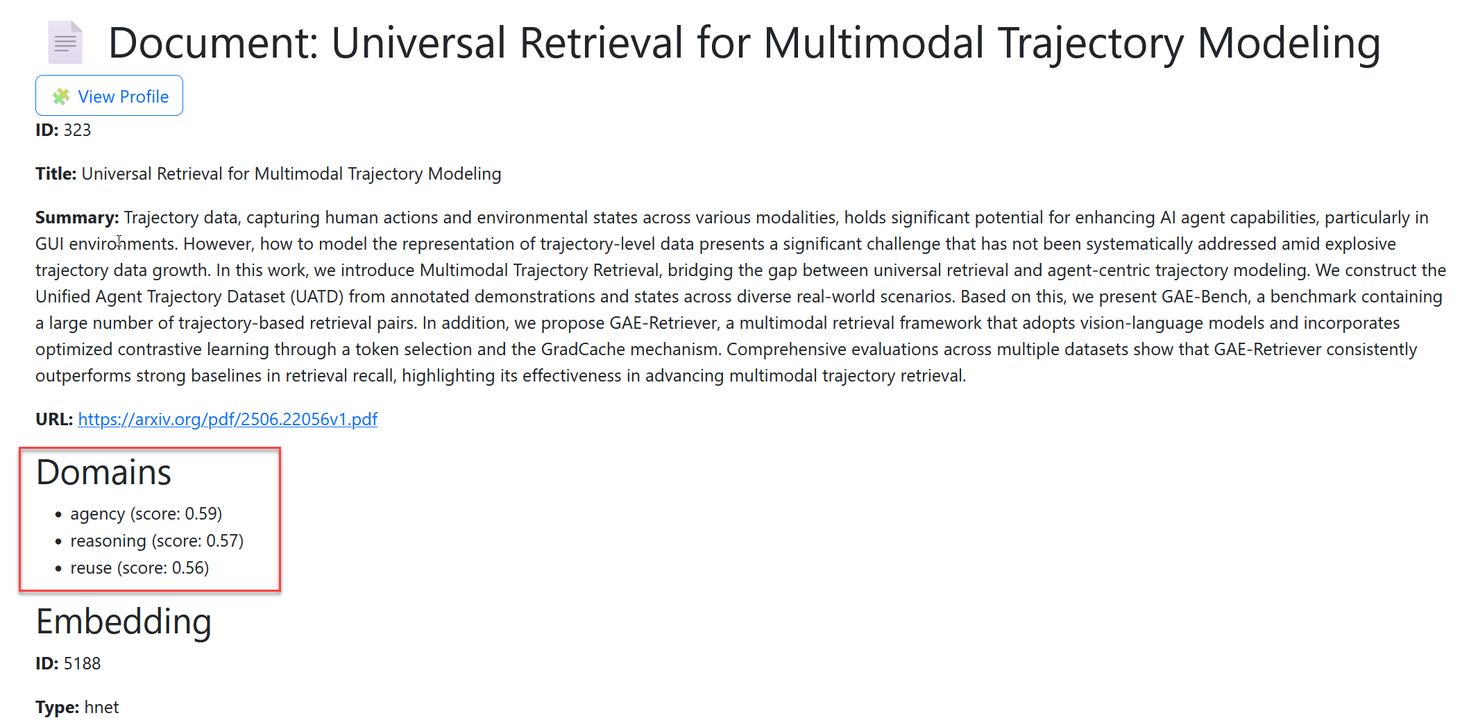 Figure showing a documentin SIS notice the domains and the related scores for the document
🌳 LATS From Scorables to Trees of Thought
Earlier we introduced the idea of the Scorable: everything in Stephanie from a document to a reasoning step can be wrapped and measured.
That abstraction becomes powerful once we realize:
- Each reasoning step can be stored as a
Scorable. - Each dimension of quality (clarity, novelty, alignment, etc.) can be applied to it.
- And reasoning itself doesn’t have to be a single line it can branch, evolve, and converge.
This is where Language Agent Tree Search (LATS) comes in.
The LATS: Language Agent Tree Search Unifies Reasoning reimagines reasoning as a tree search problem:
- Instead of one chain-of-thought, you generate multiple branches.
- Each branch is evaluated and scored.
- The system doesn’t just produce an answer, it explores a space of possibilities.
This matches perfectly with our scoring framework: every node in the tree is a Scorable.
    flowchart TD
    A[🎯 Goal] --> B[🌳 Reasoning Tree]
    B --> C1[Step 1a<br/>Scorable]
    B --> C2[Step 1b<br/>Scorable]
    C1 --> D1[Step 2a<br/>Scorable]
    C2 --> D2[Step 2b<br/>Scorable]
    D1 --> E[📊 Multi-dimensional Scoring]
    D2 --> E
🎲 Why Monte Carlo Tree Search (MCTS)?
Tree search is powerful, but it needs a way to balance:
- Exploration: trying new paths.
- Exploitation: focusing on promising paths.
That’s exactly what MCTS does. It simulates possible futures, scores them, and progressively biases toward the most rewarding paths.
For Stephanie, this means:
- Every reasoning step becomes a node (
Scorable). - Each node is scored across multiple dimensions.
- The tree grows in directions that show the most promise.
Over time, Stephanie doesn’t just answer a question she learns which reasoning strategies work best.
🧩 How It All Fits
- Scorables give us the unit of evaluation.
- LATS gives us the structure of reasoning.
- MCTS gives us the search and selection algorithm.
Together, these form the reasoning substrate that CBR will later build on because once we can generate and evaluate reasoning traces, we can start storing them as cases, retrieve them, and improve them over time.
🌳 The MCTS Reasoning Agent
At the heart of our reasoning engine is the MCTSReasoningAgent. It’s the glue that ties together:
- Monte Carlo Tree Search (MCTS) for exploring reasoning paths,
- LATS-style signatures for step generation and value estimation,
- Scorables + multidimensional evaluation for grounding every path in measurable quality.
This agent is a key piece of the system: it doesn’t just generate outputs, it explores alternatives, scores them, and learns which reasoning paths are worth following.
The full class is several hundred lines long too much to embed here. But to give you a feel for its structure, here’s a simplified, annotated version that captures the essence of how it works:
class MCTSReasoningAgent(BaseAgent):
    def __init__(self, cfg, memory, logger):
        super().__init__(cfg, memory, logger)
        self.max_depth = cfg.get("max_depth", 4)
        self.branching_factor = cfg.get("branching_factor", 2)
        self.num_simulations = cfg.get("num_simulations", 20)
        self.ucb_weight = cfg.get("ucb_weight", 1.41)
        self.dimensions = ["alignment", "clarity", "novelty", "relevance"]

    async def run(self, context: dict) -> dict:
        # 1. Start with the goal as the root of the reasoning tree
        root = self._create_node(state=context["goal"]["goal_text"], trace=[])

        # 2. Run MCTS simulations
        for _ in range(self.num_simulations):
            node = self._select(root)             # pick a promising node
            node = await self._expand(node)       # generate next steps
            reward = self._evaluate(node, context) # score the result
            self._backpropagate(node, reward)     # update tree statistics

        # 3. Return top-ranked reasoning traces as Scorables
        best_nodes = self._collect_top_k(root, k=3)
        return {"results": [self._to_scorable(n) for n in best_nodes]}

    # --- Key MCTS steps (simplified) ---
    def _select(self, node): ...
    async def _expand(self, node): ...
    def _evaluate(self, node, context): ...
    def _backpropagate(self, node, reward): ...
📝 What’s Happening Here
- Root Node: starts with the goal/problem as the root of the reasoning tree.
- Select: uses the UCT (Upper Confidence Bound) formula to balance exploration vs. exploitation.
- Expand: generates candidate next reasoning steps via DSPy/LATS.
- Evaluate: wraps each step in a
Scorable, then scores it across multiple dimensions (clarity, novelty, etc.). - Backpropagate: pushes scores back up the tree, so the search progressively favors better branches.
- Emit Results: returns the top-K reasoning traces as
Scorableobjects, ready for downstream CBR.
👉 If you want to dig deeper, the full implementation (with caching, LM budgets, value estimator hooks, and logging) is here: MCTSReasoningAgent on GitHub
    flowchart TD
    A[🎯 Goal] --> B[🌳 Root Node]
    B --> C[🔍 Select<br/>Choose promising node using UCT]
    C --> D["🌱 Expand<br/>Generate next reasoning steps (DSPy/LATS)"]
    D --> E[📏 Evaluate<br/>Score with multidimensional Scorables]
    E --> F[🔁 Backpropagate<br/>Update parent rewards & visits]
    F --> C

    E --> G[🏆 Best Paths<br/>Top-K reasoning traces as Scorables]
    G --> H[📚 Case-Based Reasoning<br/>Store & reuse best examples]

    style A fill:#f9f,stroke:#333,stroke-width:2px
    style B fill:#bbf,stroke:#333,stroke-width:1px
    style C fill:#ffd,stroke:#333,stroke-width:1px
    style D fill:#ddf,stroke:#333,stroke-width:1px
    style E fill:#cfc,stroke:#333,stroke-width:1px
    style F fill:#fcf,stroke:#333,stroke-width:1px
    style G fill:#bff,stroke:#333,stroke-width:2px
    style H fill:#fdd,stroke:#333,stroke-width:2px
🧩 Memento: Case Book Reasoning
🚪 Enter the ModularMementoAgent.
Up until now, Stephanie has been reasoning, scoring, and organizing knowledge. But she hasn’t truly learned from experience in a structured way.
The ModularMementoAgent changes that.
This is our first agent built around case-based reasoning (CBR). Instead of treating each run as an isolated event, it remembers past cases, compares them with new ones, and gradually refines its approach.
Think of it as giving Stephanie her first long-term memory system for reasoning where every trace, hypothesis, and decision is turned into a “case” that can be retrieved, reused, revised, and retained.
To see how this fits together, here’s the map we’ll follow for the rest of this section:
    flowchart TD
    A[🎯 Goal + Context] --> B[🤖 ModularMementoAgent]
    B --> C["MCTSReasoningAgent<br/>Base Run (Generates Scorables)"]
    C --> D[CBR Middleware]

    subgraph D[🧩 CBR Middleware]
        D1[📂 ContextNamespacer]
        D2[📖 CasebookScopeManager]
        D3[🔍 CaseSelector]
        D4["📊 Rank & Analyze<br/>(ScorableRanker + MARS)"]
        D5[✅ QualityAssessor]
        D6[🏆 ChampionPromoter]
        D7[📝 GoalStateTracker]
        D8[⚖️ ABValidator]
        D9[🧠 MicroLearner]
        D10[📦 RetentionPolicy]
    end

    D1 --> D2 --> D3 --> D4 --> D5 --> D6 --> D7 --> D8 --> D9 --> D10
    D10 --> E["(💾 Casebook Storage)"]

    E -->|Retrieve Past Cases| D3
    D4 -->|Ranked Outputs| B
At the code level, the agent looks like this:
class ModularMementoAgent(MCTSReasoningAgent):
    def __init__(self, cfg, memory, logger):
        super().__init__(cfg, memory, logger)

        # Wire together all CBR middleware components
        ns = DefaultContextNamespacer()
        scope = DefaultCasebookScopeManager(cfg, memory, logger)
        selector = DefaultCaseSelector(cfg, memory, logger)
        ranker = DefaultRankAndAnalyze(cfg, memory, logger,
            ranker=ScorableRanker(cfg, memory, logger),
            mars=MARSCalculator(cfg, memory, logger) if cfg.get(INCLUDE_MARS, True) else None)
        retention = DefaultRetentionPolicy(cfg, memory, logger, casebook_scope_mgr=scope)
        assessor = DefaultQualityAssessor(cfg, memory, logger)
        promoter = DefaultChampionPromoter(cfg, memory, logger)
        tracker = DefaultGoalStateTracker(cfg, memory, logger)
        ab = DefaultABValidator(cfg, memory, logger, ns=ns, assessor=assessor)
        micro = DefaultMicroLearner(cfg, memory, logger)

        # Assemble into a single middleware pipeline
        self._cbr = CBRMiddleware(cfg, memory, logger,
                                  ns, scope, selector, ranker,
                                  retention, assessor, promoter,
                                  tracker, ab, micro)

    async def run(self, context: dict) -> dict:
        # Connect middleware with the base reasoning agent (MCTS)
        self._cbr.ranker.scoring = self.scoring
        parent_run = super(ModularMementoAgent, self).run

        async def base_run(ctx):
            return await parent_run(ctx)

        context[AGENT_NAME] = self.name
        return await self._cbr.run(context, base_run, self.output_key)
📌 Key idea: this class is just the wiring harness. It connects our familiar MCTSReasoningAgent to the new CBR middleware, so every run is now guided by past cases and reinforced by quality checks.
👉 Next, we’ll follow the diagram step by step starting with the ContextNamespacer, the small but vital piece that keeps every case organized in its proper scope.
📂 ContextNamespacer: Keeping Cases in Their Lanes
When you start remembering everything, chaos is a real risk. Without structure, cases from one goal could spill over into another, or context from one pipeline run could contaminate another.
The ContextNamespacer solves this by acting as a namespace manager for reasoning traces. It ensures that every case whether it’s a hypothesis, a document, or a scored trace is tagged with the right scope and separated cleanly.
Think of it as the filing cabinet labels for Stephanie’s case memory:
- 🗂️ Goal Namespace ties each case to the specific goal it was created under.
- 🧩 Run Namespace distinguishes cases produced in different reasoning runs.
- 🔑 Scoped IDs creates consistent keys so scorables, embeddings, and results can be linked back unambiguously.
Without namespacing:
- A “clarity” score from one goal might get mixed with an “alignment” score from another.
- A reasoning trace about vision models might pollute the retrieval set when working on symbolic planning.
With namespacing:
- Every case is contained in the right scope, making retrieval and reuse safe.
- The CBR middleware can operate across thousands of runs without collisions.
🧭 Flow in the Middleware
    flowchart LR
    A[🎯 Goal + Context] --> B[📂 ContextNamespacer]
    B --> C[📖 CasebookScopeManager]

    style B fill:#e6f7ff,stroke:#0077b6,stroke-width:2px
    style A fill:#f9f,stroke:#333,stroke-width:2px
    style C fill:#bbf,stroke:#333,stroke-width:2px
The ContextNamespacer is the very first step in the pipeline. Before we even think about retrieving or ranking, it stamps each case with the right identifiers so all downstream modules know where it belongs.
⌨️ In Code Terms
The implementation is simple but foundational:
class DefaultContextNamespacer:
    def make_scoped_id(self, goal_id: str, case_id: str) -> str:
        """Attach goal context to a case id."""
        return f"{goal_id}::{case_id}"

    def extract_scope(self, scoped_id: str) -> Tuple[str, str]:
        """Split back into (goal_id, case_id)."""
        return tuple(scoped_id.split("::", 1))
Every Scorable that passes through the system can now be unambiguously tied back to the goal and run that created it.
👉 Next up: the CasebookScopeManager, which uses these namespaces to decide which casebooks to search and update when a new reasoning run begins.
📖 CasebookScopeManager: Defining the Boundaries of Memory
If the ContextNamespacer gives each case a label, the CasebookScopeManager decides which shelf in the library it belongs to.
The system doesn’t just have one big bucket of cases. Instead, cases are grouped into casebooks structured collections of past reasoning tied to goals, domains, or experiments.
The CasebookScopeManager answers questions like:
- 📚 Which casebook should this new case be added to?
- 🔍 When I want to retrieve past knowledge, which casebooks should I search?
- 🧭 How do we keep the scope small enough to be relevant, but broad enough to be useful?
🚷 Boundaries to our knowledge
Without scope management:
- Retrieval might trawl across unrelated casebooks, pulling in irrelevant or noisy cases.
- Updates could end up in the wrong memory, confusing future reasoning.
With a CasebookScopeManager:
- Every run has a clear boundary of which casebooks are in play.
- Memory remains organized, relevant, and efficient.
🧭 Flow in the Middleware
    flowchart LR
    A[📂 ContextNamespacer] --> B[📖 CasebookScopeManager]
    B --> C[🔍 CaseSelector]

    style B fill:#fef9e7,stroke:#b8860b,stroke-width:2px
    style A fill:#e6f7ff,stroke:#0077b6,stroke-width:2px
    style C fill:#bbf,stroke:#333,stroke-width:2px
The CasebookScopeManager acts like the traffic controller between raw namespaces and the retrieval engine. It says:
“Given this goal and context, here are the casebooks you’re allowed to look at and update.”
💻 In Code Terms
The real implementation is more involved, but the essence looks like this:
class DefaultCasebookScopeManager:
    def __init__(self, cfg, memory, logger):
        self.cfg, self.memory, self.logger = cfg, memory, logger

    def active_casebooks(self, goal_id: str) -> list:
        """Return the casebooks relevant for this goal."""
        return self.memory.casebooks.find_for_goal(goal_id)

    def ensure_casebook(self, goal_id: str, description="") -> str:
        """Guarantee a casebook exists for this goal, return its id."""
        return self.memory.casebooks.ensure(goal_id, description)
🔑 Key Role
The CasebookScopeManager ensures:
- 🏷️ New cases are stored in the right casebook.
- 📖 Retrieval queries are focused on relevant casebooks.
- 🔄 Updates don’t bleed across unrelated goals.
👉 Next, we’ll step into the CaseSelector the module that decides which cases to pull back out once the scope has been defined.
🔍 CaseSelector: Choosing Which Memories to Reuse
Once the CasebookScopeManager has told us where to look, the CaseSelector decides what to pull back out.
Think of it as the retrieval engine of the CBR pipeline. Its job is to balance:
- 🏆 High-quality cases (champions from past reasoning).
- 🕒 Recent successes (things that worked well last time).
- 🎲 Novel or diverse candidates (to avoid overfitting to the same cases).
- 🎯 Exploration (injecting fresh possibilities).
🏅 Best of the best
Without selection pressure, Stephanie could drown in irrelevant or redundant past cases. The CaseSelector makes sure the system always has a curated set of candidates for reuse a balance between stability and exploration.
⚖️ Selection Strategy
Here’s the rough strategy used by the default implementation:
-
Champion-first If a case has proven itself as the champion for a goal, reuse it first.
-
Recent-success Bring in the most recent accepted cases they reflect what’s currently working.
-
Diverse-novel Add candidates that are different from what we’ve already picked.
-
Exploration Randomly toss in a few extra cases sometimes the best ideas come from unexpected sources.
🧭 Flow in the Middleware
    flowchart LR
    A[📖 CasebookScopeManager] --> B[🔍 CaseSelector] --> C[📊 Rank & Analyze]
    style B fill:#f9f9f9,stroke:#333,stroke-width:2px
The CaseSelector doesn’t make the final decision on what’s best it just assembles a shortlist of reuse candidates to be scored, ranked, and analyzed in the next step.
🧑 In Code Terms
The actual implementation is bigger, but the heart of it looks like this:
class DefaultCaseSelector:
    def __init__(self, cfg, memory, logger):
        self.cfg, self.memory, self.logger = cfg, memory, logger

    def build_reuse_candidates(self, casebook_id, goal_id, cases, budget=10):
        candidates = []

        # 1. Champion-first
        champion = self.memory.casebooks.get_champion(casebook_id, goal_id)
        if champion:
            candidates.append(champion)

        # 2. Recent-success
        recent = self.memory.casebooks.get_recent_successes(casebook_id, goal_id, limit=3)
        candidates.extend(recent)

        # 3. Diverse-novel
        pool = self.memory.casebooks.get_novel_pool(casebook_id, goal_id, exclude=candidates)
        candidates.extend(pool[:2])

        # 4. Exploration (random injection)
        if random.random() < 0.2:
            candidates.extend(random.sample(cases, 2))

        return candidates[:budget]
🔑 Key Role
The CaseSelector ensures that every reasoning run has a diverse but relevant set of prior cases to draw inspiration from.
It doesn’t decide the winner it feeds candidates into the ranking system that comes next.
👉 Next, we’ll cover the Rank & Analyze stage, where those candidates are actually evaluated and compared.
📊 Rank & Analyze: Enhanced Scoring for Smarter Case Reuse
Once cases are retrieved, Stephanie can’t just accept them at face value. She needs to evaluate them across multiple dimensions, using multiple scorers, and with checks for consistency.
That’s the role of Rank & Analyze, powered by:
- ScorableRanker – computes a weighted, multi-signal score for each candidate.
- MARS (Model Agreement & Reasoning Signal) – validates whether those scores are trustworthy.
🧮 ScorableRanker: Weighted, Multi-Signal Case Scoring
The ScorableRanker extends traditional similarity ranking with richer signals inspired by CBR research. Instead of just “how close is this case to the goal?”, it combines:
- Similarity (goal ↔ case embedding match).
- Value (past reward signals from evaluations).
- Recency (cases fade over time via exponential decay).
- Diversity (Maximal Marginal Relevance avoid clones of already picked cases).
- Adaptability (does this case generalize? Does it use tools available in the current context?).
components = {
    "similarity": self._similarity(query_emb, cand_emb),
    "value": self._value(cand),
    "recency": self._recency(cand),
    "adaptability": self._adaptability(cand, context),
    "diversity": self._diversity(cand, selected),
}
rank_score = sum(
    components[k] * self.weights.get(k, 0) for k in components
)
By default, weights are inspired by CBR literature (similarity 0.45, value 0.30, recency 0.10, diversity 0.10, adaptability 0.05).
🔑 Takeaway: Instead of a flat “nearest neighbor” score, cases now have a composite rank score that balances short-term similarity, long-term value, and contextual adaptability.
🌌 MARS: Measuring Agreement and Reliability
The MARSCalculator goes one step deeper. It looks across all scorers (MRQ, SICQL, EBT, LLM) and asks:
- Do they agree on which cases are good?
- If not, where’s the conflict?
- Which scorer is most reliable given our trust reference (e.g., LLM)?
result = {
    "dimension": str(dimension),
    "agreement_score": 0.87,   # 1 - variance
    "std_dev": 0.12,           # disagreement spread
    "preferred_model": "ebt",  # closest to trust reference
    "primary_conflict": ["mrq", "llm"],
    "delta": 0.22,             # difference between top & bottom
    "high_disagreement": False,
    "explanation": "MARS agreement: 0.87 | Most aligned with llm: ebt | Primary conflict: mrq vs llm (Δ=0.22)",
}
MARS reports include:
- Agreement Score: normalized consensus (1 = perfect agreement, 0 = chaos).
- Primary Conflict: biggest scorer disagreement (e.g., MRQ vs LLM).
- Preferred Model: scorer most aligned with the trust reference.
- Diagnostics: explanations, correlations between metrics, and reliability estimates.
⚡ Worked Example
Let’s say the goal is:
“Evaluate new planning strategies in symbolic reasoning.”
We retrieve 3 candidate cases:
| Case | Similarity | Value | Recency | Diversity | Adaptability | Rank Score | MARS Agreement | Conflict |
|---|---|---|---|---|---|---|---|---|
| A | 0.92 | 0.81 | 0.95 | 0.80 | 0.70 | 0.86 | High (0.91) | None |
| B | 0.75 | 0.60 | 0.70 | 0.65 | 0.85 | 0.73 | Medium (0.72) | MRQ vs LLM |
| C | 0.58 | 0.92 | 0.40 | 0.95 | 0.55 | 0.69 | Low (0.51) | EBT vs LLM |
📌 Interpretation:
- Case A → Strong all-rounder, high trust.
- Case B → Adaptable but contested (scorers disagree).
- Case C → Novel but risky (MARS shows low agreement).
📐 Flow in Middleware
    flowchart TD
    A[🔍 Retrieved Cases] --> B[📊 ScorableRanker<br/>Composite Scoring]
    B --> C[🌌 MARS<br/>Agreement + Conflict Analysis]
    C --> D[✅ QualityAssessor<br/>Keep or Discard?]
    D --> E[🏆 ChampionPromoter<br/>Best Case to Champion]
🚀 Deep understanding
The combination of ScorableRanker + MARS is one of the core contributions of this system:
- Stephanie no longer just finds “nearest cases.”
- She ranks them based on multiple signals relevant to reasoning.
- She validates them with agreement checks before trusting them.
This is what makes the ModularMemento pipeline robust: it’s not just memory, it’s measured, trustworthy memory.
Perfect 👍 if you’re planning to show real MARS output screenshots in SIS, then this section is where we really roll up our sleeves and explain exactly what MARS is doing under the hood. That way the visuals will have maximum impact.
Here’s how I’d structure the deep-dive:
🌌 Inside MARS: Measuring Agreement and Reasoning Signal
The MARSCalculator (Model Agreement & Reasoning Signal) is the engine that tells us whether to trust our scoring results.
Where the ScorableRanker evaluates candidates, MARS evaluates the evaluators themselves. It asks:
- Do the scorers agree on what’s good?
- If not, who do we trust?
- Where are the conflicts and weak signals that deserve human review?
🧭 Step 1: Per-Dimension Analysis
Every document, hypothesis, or case is scored along multiple dimensions (e.g., clarity, novelty, alignment). MARS operates within each dimension separately, ensuring we understand not just how good a case is overall, but how reliable scoring is in that specific dimension.
    flowchart TD
    A[📂 ScoreCorpus] --> B["📏 Dimension Matrix<br/>(docs × scorers)"]
    B --> C[📊 Agreement & Variance Analysis]
    B --> D[⚔️ Conflict Detection]
    B --> E[🎯 Preferred Model Selection]
    C & D & E --> F[🌌 MARS Result per Dimension]
📊 Agreement & Variance
- Std. Deviation: How much scorers diverge on this dimension.
- Agreement Score:
1 - variance(normalized between 0 and 1).
👉 High agreement = safe to trust. 👉 High variance = risky dimension.
# Agreement = 1 - std deviation
agreement_score = max(0.0, min(1.0, 1.0 - float(std_dev)))
⚔️ Conflict Detection
MARS finds the biggest disagreement between scorers:
scorer_means = col_means.fillna(0.0)
max_name = scorer_means.idxmax()
min_name = scorer_means.idxmin()
delta = scorer_means[max_name] - scorer_means[min_name]
primary_conflict = [max_name, min_name]
Example:
- MRQ avg = 0.82
- LLM avg = 0.61
- Conflict = MRQ vs LLM (Δ = 0.21)
This tells us where scorers see the world differently.
🎯 Preferred Model Selection
Who should we trust when scorers disagree?
MARS compares every scorer’s outputs against a trust reference (default: LLM). The model whose scores are closest to the trust reference is marked as preferred.
for scorer in matrix.columns:
    diff = (matrix[scorer] - trust_scores).abs().mean()
    if diff < min_diff:
        preferred_model = scorer
If no trust reference exists, MARS defaults to the median scorer.
📈 Scorer Reliability
MARS also tracks reliability per scorer either by correlation with the trust reference or by how consistent a scorer is across docs.
| Scorer | Reliability |
|---|---|
| LLM | 1.00 (reference) |
| MRQ | 0.78 |
| EBT | 0.82 |
| SVM | 0.66 |
This lets us spot when one scorer drifts or collapses.
🧠 Human-Readable Explanation
Every MARS result includes a narrative explanation for logs & dashboards:
{
  "dimension": "clarity",
  "agreement_score": 0.87,
  "preferred_model": "ebt",
  "primary_conflict": ["mrq", "llm"],
  "delta": 0.22,
  "explanation":
    "MARS agreement: 0.87 | Most aligned with llm: ebt | Primary conflict: mrq vs llm (Δ=0.22)"
}
This is what you’ll see visualized in SIS reports.
📚 Example MARS Report
Let’s say we ran MARS across 3 dimensions:
| Dimension | Agreement | Conflict | Preferred | Explanation |
|---|---|---|---|---|
| Clarity | 0.91 | None | MRQ | High agreement, MRQ best aligned |
| Novelty | 0.68 ⚠️ | LLM vs SVM | EBT | Disagreement flagged (Δ=0.25) |
| Alignment | 0.79 | MRQ vs LLM | MRQ | Moderate agreement |
📌 Interpretation:
- Clarity → safe to trust.
- Novelty → high risk, needs review.
- Alignment → some disagreement, but MRQ aligns with LLM.
🔮 Making sense of scores everywhere
Without MARS, Stephanie would blindly trust whichever model gave a score. With MARS, she can:
- Detect hidden disagreements.
- Choose the most reliable scorer automatically.
- Flag contentious dimensions for review.
- Build a transparent audit trail of every decision.
🖼️ MARS in Action
Here’s what a MARS report looks like inside the SIS dashboard. Each bar and row reflects how scorers performed on a single pipeline run:
- Agreement score shows how much the models aligned.
- Preferred model highlights which scorer is most trustworthy.
- Conflicts are flagged clearly for human review.
    flowchart TD
    A[Pipeline Run] --> B[📊 MARS Dashboard]
    B --> C[✅ Agreement Score]
    B --> D[🎯 Preferred Model]
    B --> E[⚔️ Conflict Detection]
    B --> F[🧾 Explanation]
📸 Screenshot below: A real SIS pipeline, with MARS surfacing scorer agreement, highlighting conflicts, and pointing to the most reliable model.
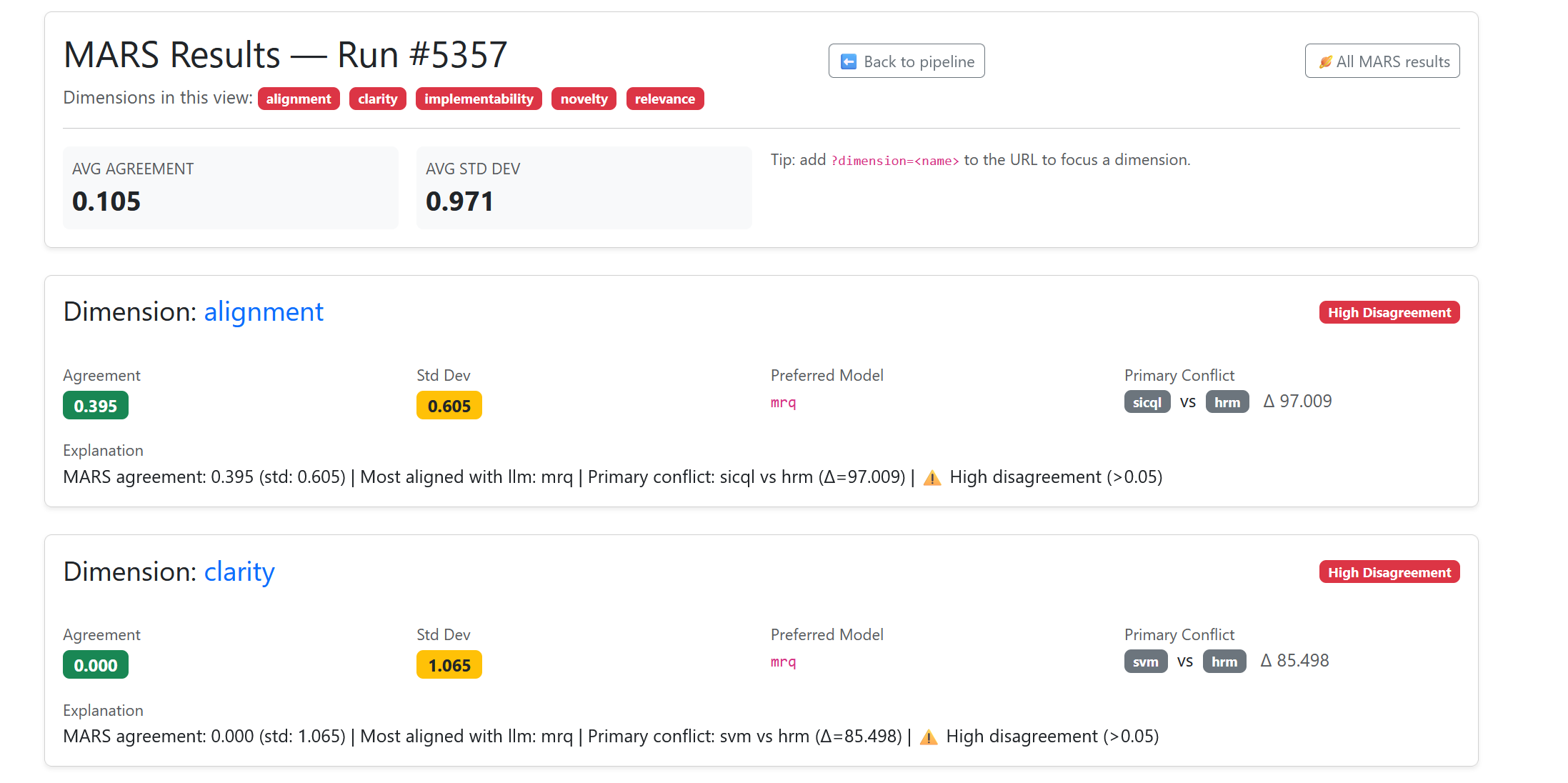
✓ In summary: MARS tells us if our scorers agree. High agreement means we can trust the result. Low agreement flags a decision for review. This makes our CBR loop robust and auditable.
✅ Assessing Case Quality
Not every reasoning path or output is worth keeping. Some are noisy, misleading, or simply irrelevant. That’s why Stephanie has a Quality Assessor module built directly into the CBR loop.
The Quality Assessor acts like a filter between ranked scorables and the casebook:
- 🧹 Filters out weak cases – only high-quality candidates survive.
- 🎯 Checks for alignment with goals – making sure what we retain is actually useful.
- 🔄 Standardizes evaluations – turning diverse scores and signals into a consistent “quality verdict.”
    flowchart LR
    A[Ranked Scorables] --> B[✅ Quality Assessor]
    B -->|Pass| C[🏆 Champion Promoter]
    B -->|Fail| D[🗑️ Discard / Ignore]
This step is crucial. Without a quality filter, the casebook would quickly fill up with clutter making retrieval noisy and learning less effective. With it, Stephanie ensures that only the best examples shape future reasoning.
🧹 The Quality Assessor in Action
At its core, the Quality Assessor takes a candidate Scorable (document, reasoning path, hypothesis, etc.) and decides if it’s good enough to keep.
Here’s the code:
class DefaultQualityAssessor:
    def __init__(self, cfg, memory, logger):
        self.cfg = cfg
        self.memory = memory
        self.logger = logger
        self.threshold = float(cfg.get("quality_threshold", 0.6))

    def assess(self, scorable: Dict[str, Any]) -> bool:
        """
        Decide whether a scorable is "good enough" to be retained.
        Returns True if passed, False if rejected.
        """
        try:
            score = scorable.get("rank_score") or 0.0
            meta = scorable.get("components", {})

            # Basic threshold check
            if score < self.threshold:
                self.logger.log("QualityReject", {
                    "id": scorable.get("id"),
                    "score": score,
                    "reason": f"Below threshold {self.threshold}"
                })
                return False

            # Optional: penalize very low clarity or alignment
            clarity = meta.get("clarity", 1.0)
            alignment = meta.get("alignment", 1.0)

            if clarity < 0.3 or alignment < 0.3:
                self.logger.log("QualityReject", {
                    "id": scorable.get("id"),
                    "clarity": clarity,
                    "alignment": alignment,
                    "reason": "Critical dimension below threshold"
                })
                return False

            # Passed quality checks
            self.logger.log("QualityAccept", {
                "id": scorable.get("id"),
                "score": score,
                "clarity": clarity,
                "alignment": alignment
            })
            return True

        except Exception as e:
            self.logger.log("QualityAssessorError", {"error": str(e)})
            return False
🔍 What’s Happening Here
-
Threshold Gate
- Every scorable gets a
rank_score. If it’s below the configuredquality_threshold(default = 0.6), it’s rejected immediately.
- Every scorable gets a
-
Dimension Safety Checks
- Even if the rank score is good, we don’t want cases with glaring weaknesses.
- For example, if clarity or alignment scores are critically low (<0.3), the case is discarded.
-
Structured Logging
- Every accept/reject is logged with reasons, so we can later audit why a case was filtered.
🚮 Dump the trash
Without this filter, Stephanie would store everything, including:
- Noisy reasoning traces that confuse later retrieval.
- Low-value outputs that waste training cycles.
- Misaligned or ambiguous results that derail future reasoning.
By enforcing a quality gate, we ensure that the casebook evolves toward excellence:
- Only good enough cases get retained.
- Retrieval is cleaner and more precise.
- Learning loops are powered by high-signal, low-noise examples.
🏆 Champion Promoter: Remembering the Best
Once we’ve filtered out the noise with the Quality Assessor, we don’t just want to keep all acceptable cases. Some are better than others and the system needs to know its current best example for each goal.
That’s the role of the Champion Promoter.
It tracks which case currently holds the title of “champion” for a given goal, and promotes new challengers only when they outperform the existing one.
☸️ We know what we know
- Keeps a single source of truth for the best-known solution per goal.
- Prevents “casebook bloat” with too many near-duplicates.
- Enables downstream modules (like the Case Selector) to prioritize high-quality seeds.
🧩 Example Code (simplified)
class DefaultChampionPromoter:
    def __init__(self, cfg, memory, logger):
        self.cfg, self.memory, self.logger = cfg, memory, logger

    def promote(self, goal_id: str, candidate: dict) -> bool:
        """
        Try to promote a candidate as the new champion for this goal.
        Returns True if promotion happened, False otherwise.
        """
        current = self.memory.casebooks.get_champion(goal_id)

        # No champion yet → auto-promote
        if not current:
            self.memory.casebooks.set_champion(goal_id, candidate)
            self.logger.log("ChampionPromoted", {
                "goal": goal_id, "id": candidate.get("id"), "reason": "First champion"
            })
            return True

        # Compare rank_score (or other metrics)
        if candidate.get("rank_score", 0) > current.get("rank_score", 0):
            self.memory.casebooks.set_champion(goal_id, candidate)
            self.logger.log("ChampionPromoted", {
                "goal": goal_id, "id": candidate.get("id"), "reason": "Outperformed old champion"
            })
            return True

        # Candidate not better
        self.logger.log("ChampionNotPromoted", {
            "goal": goal_id, "id": candidate.get("id"), "reason": "Did not beat champion"
        })
        return False
⚡ The Effect
The Champion Promoter acts like a tournament bracket:
- Every new candidate competes with the reigning champion.
- Only if it beats the champion does it replace it.
- This ensures a constant upward trajectory in case quality.
    flowchart LR
    A[📊 Candidate Case] --> B[✅ Quality Assessor]
    B -->|Passes| C[🏆 Champion Promoter]
    B -->|Fails| X[❌ Discarded]

    C -->|Beats Champion| D[⭐ New Champion Stored]
    C -->|Not Better| E[↩️ Champion Retained]

    D --> F[📝 Goal State Tracker]
    E --> F

    F --> G[(💾 Casebook DB)]
    G --> H[📂 Used by Case Selector for Future Runs]
🔑 How to read this:
- Only quality-approved cases reach the Champion Promoter.
- The promoter ensures that only the best candidate per goal survives as champion.
- The Goal State Tracker keeps everything consistent in the database so that the Case Selector always knows where to start.
📝 Goal State Tracker: Remembering the Champion
So far, we’ve seen how new cases are scored, assessed for quality, and possibly promoted as champions. But for a self-improving system, it’s not enough to pick a winner in the moment we need to remember that winner across future runs.
That’s the job of the Goal State Tracker.
🏦 What It Does
- Keeps a record of the current champion for each
(goal, casebook)pair. - Updates the champion when the Champion Promoter signals a new best case.
- Stores metadata like when it was promoted, why it was promoted, and its key scorable signals.
- Provides fast retrieval for the Case Selector, so the system can start from its best-known solution instead of reinventing the wheel.
This is essentially the “memory cell” for CBR the point where experience becomes institutional knowledge.
🔎 Example: Champion Persistence
class GoalStateTracker:
    def __init__(self, memory, logger):
        self.memory = memory
        self.logger = logger

    def update_champion(self, casebook_id: int, goal_id: str, case_id: str):
        """
        Set the given case as the champion for this goal.
        """
        self.memory.casebooks.set_champion(casebook_id, goal_id, case_id)
        self.logger.log(
            "ChampionUpdated",
            {"casebook_id": casebook_id, "goal_id": goal_id, "new_champion": case_id},
        )

    def get_champion(self, casebook_id: int, goal_id: str):
        """
        Retrieve the current champion case for this goal.
        """
        return self.memory.casebooks.get_champion(casebook_id, goal_id)
🪢 Learn from history
Without the tracker, the agent would forget its hard-earned lessons. By explicitly recording champions:
- Future runs can bootstrap from proven successes.
- We can analyze how champions evolve over time.
- The system becomes self-stabilizing: bad cases don’t overwrite champions unless they’re clearly better.
Great let’s tackle the A/B Validator section. This is where the system stops being theoretical and actually tests alternatives head-to-head before updating memory.
⚖️ A/B Validator: Putting Cases to the Test
Promoting a new champion is a big deal. If we do it too eagerly, we risk forgetting good solutions. If we do it too conservatively, we miss out on better ones.
The A/B Validator exists to strike that balance.
🧠 What It Does
- Takes a candidate case (the challenger) and compares it to the current champion.
- Uses the same scoring engines (ScorableRanker, MARS, etc.) across multiple dimensions.
- Decides whether the challenger is truly better before updating the Goal State Tracker.
- Records the evaluation so that results are transparent and reproducible.
🧪 Example: Challenger vs Champion
class ABValidator:
    def __init__(self, assessor, logger):
        self.assessor = assessor
        self.logger = logger

    def validate(self, champion, challenger, context):
        """
        Compare champion vs challenger.
        Return True if challenger should replace champion.
        """
        champ_score = self.assessor.assess(champion, context)
        chall_score = self.assessor.assess(challenger, context)

        better = chall_score > champ_score
        self.logger.log(
            "ABValidation",
            {
                "champion_score": champ_score,
                "challenger_score": chall_score,
                "winner": "challenger" if better else "champion",
            },
        )
        return better
🎯 Prove it
This step ensures that:
- Champions aren’t overwritten unless the challenger proves itself.
- We can experiment safely without destabilizing the system.
- Validation logs give us a paper trail of improvements we can see when, how, and why a champion was replaced.
In short: the A/B Validator makes sure our agent’s evolution is based on evidence, not hype.
👉 Next up in the Mermaid diagram is the MicroLearner the component that takes these validation results and squeezes extra training signal out of them.
🧠 MicroLearner: Learning in the Small
Big retraining loops are expensive. They require lots of data, time, and compute. But what if we could learn incrementally, case by case, as new evidence comes in?
That’s the role of the MicroLearner.
⚙️ What It Does
-
Watches the results of each CBR cycle (champions, challengers, validation outcomes).
-
Extracts tiny training signals from every decision:
- “This case scored higher than that one.”
- “This output was accepted, that one was discarded.”
-
Converts those signals into on-the-fly updates for scorers (MRQ, EBT, SVM, etc.).
-
Keeps models fresh and adaptive without waiting for full retrains.
Think of it as fine-grained gradient nudges that happen inside the reasoning loop.
🔍 Example: Online Update
Here’s a simplified sketch of how it works:
class MicroLearner:
    def __init__(self, memory, logger):
        self.memory = memory
        self.logger = logger

    def update_from_validation(self, champion, challenger, result):
        """
        Tiny supervised update: reward the winner, penalize the loser.
        """
        if result == "challenger":
            self._reward(challenger, 1.0)
            self._reward(champion, 0.0)
        else:
            self._reward(champion, 1.0)
            self._reward(challenger, 0.0)

    def _reward(self, case, reward_value):
        self.memory.rewards.add(
            case_id=case.id,
            reward=reward_value,
        )
        self.logger.log(
            "MicroUpdate",
            {"case_id": case.id, "reward": reward_value},
        )
🚀 Why It Matters
- Always learning: Every decision provides feedback.
- Low overhead: Updates happen instantly, without pausing for retraining jobs.
- Better over time: Even small nudges accumulate into significant improvements.
In other words, the MicroLearner makes sure Stephanie never wastes an experience every case, win or lose, sharpens the system.
    flowchart TD
    A[🏆 Champion Case] --> C[⚖️ AB Validation]
    B[🥊 Challenger Case] --> C

    C -->|Winner/Loser| D[🧠 MicroLearner]

    subgraph D[MicroLearner]
        D1[📊 Compare outcomes]
        D2[✏️ Assign rewards<br/>Champion vs Challenger]
        D3[🔄 Online update<br/>Scoring Models]
    end

    D --> E["📈 Scorers (MRQ, EBT, SVM)"]
    E --> F[💡 Improved Future Ranking]

    style A fill:#bbf,stroke:#333,stroke-width:1px
    style B fill:#fbb,stroke:#333,stroke-width:1px
    style C fill:#ffd,stroke:#333,stroke-width:1px
    style D fill:#dfd,stroke:#333,stroke-width:2px
    style E fill:#cfc,stroke:#333,stroke-width:1px
    style F fill:#fcf,stroke:#333,stroke-width:2px
📦 After the MicroLearner comes the Retention Policy, which decides how long cases stick around and which ones fade out.
📦 Retention Policy: Deciding What to Keep
Not every case is worth saving. Some are noisy, redundant, or outright harmful. The Retention Policy makes sure Stephanie’s casebooks don’t just grow endlessly they evolve with quality in mind.
🔍 What It Does
-
Filters cases before they’re stored in the casebook.
-
Applies rules & thresholds (like minimum score, novelty, or domain balance).
-
Decides retention mode:
- ✅ Accept: store permanently.
- ⏳ Stash: keep temporarily for review.
- ❌ Reject: discard outright.
-
Logs the decision so we know why something was kept or dropped.
This keeps the system lean, adaptive, and bias-aware. Without it, CBR would just hoard everything.
🧠 Why It Matters
CBR depends on the quality of its memory. If bad or redundant cases stick around, retrieval gets noisy and reasoning degrades.
The Retention Policy ensures:
- 📉 Noise control we don’t clutter the casebook.
- 🧬 Novelty preservation genuinely new cases make it in.
- 🎯 Goal alignment cases must actually help the agent.
Think of it as Marie Kondo for AI memory:
If a case doesn’t spark learning, it doesn’t stay.
⚙️ A Simplified Example
Here’s a slimmed-down code snippet from retention_policy.py that shows the essence:
class DefaultRetentionPolicy:
    def __init__(self, cfg, memory, logger, casebook_scope_mgr):
        self.cfg = cfg
        self.memory = memory
        self.logger = logger
        self.scope_mgr = casebook_scope_mgr

    def should_retain(self, case) -> str:
        """
        Decide what to do with a case:
        return "accept", "stash", or "reject".
        """
        score = case.get("score", 0.0)
        novelty = case.get("novelty", 0.0)

        if score < 0.3:
            return "reject"
        elif novelty < 0.1:
            return "stash"
        return "accept"
🔁 Where It Fits
Let’s place it in context with the full CBR loop:
    flowchart LR
    A[📄 New Case] --> B[📊 Rank & Analyze]
    B --> C[✅ Quality Assessor]
    C --> D[🏆 Champion/Challenger]
    D --> E[⚖️ AB Validator]
    E --> F[🧠 MicroLearner]
    F --> G[📦 Retention Policy]
    G -->|Accept| H[(💾 Casebook Storage)]
    G -->|Reject/Stash| I[🗑️ Drop or Hold]

    style G fill:#ffd,stroke:#333,stroke-width:2px
    style H fill:#cfc,stroke:#333,stroke-width:2px
This diagram shows:
- Cases are only written to the Casebook after passing through Retention Policy.
- Everything else (scoring, validation, micro-learning) feeds into this gate.
✅ With Retention Policy, Stephanie’s casebooks don’t just grow they curate themselves.
Great question this is where we can make the post more concrete and also show the power of Retention Policy. Right now we only hinted at the simplest form (keep if score > 0.3, novelty > 0.1). But in practice, we layer rules that reflect how a case contributes to long-term learning.
Here’s how you could explain it in the blog:
📐 Retention Rules: Curating Memory for Growth
The Retention Policy isn’t a one-size-fits-all filter it applies multiple rules to decide whether a case strengthens the casebook or just adds noise.
⚖️ Examples of Rules
-
Score Thresholds
- Reject cases that don’t meet a minimum quality score (e.g., clarity < 0.3).
- Ensures we don’t store junk.
-
Novelty & Diversity
- Penalize cases that are too similar to existing ones.
- Encourage retention of genuinely new reasoning paths.
-
Domain Balance
- If a casebook is over-saturated in one domain (e.g., 80% “planning”), reject or stash new cases from that domain.
- Keeps knowledge coverage broad.
-
Temporal Freshness
- Prioritize recent cases when concepts are evolving fast.
- Optionally prune stale cases after N days.
-
Goal Alignment
- Check if the case actually advances the current goal.
- Even a high-scoring case might be irrelevant to the task at hand.
🧩 Putting It Together
Here’s a more detailed (but still readable) policy function:
class DefaultRetentionPolicy:
    def __init__(self, cfg, memory, logger, casebook_scope_mgr):
        self.cfg = cfg
        self.memory = memory
        self.logger = logger
        self.scope_mgr = casebook_scope_mgr

    def should_retain(self, case) -> str:
        score = case.get("score", 0.0)
        novelty = case.get("novelty", 0.0)
        domain = case.get("domain", "unknown")
        age_days = case.get("age_days", 0)

        # Rule 1: basic quality gate
        if score < 0.3:
            return "reject"

        # Rule 2: novelty encourages learning
        if novelty < 0.1:
            return "stash"  # don’t delete, but don’t commit

        # Rule 3: domain balancing
        if self.scope_mgr.domain_overloaded(domain):
            return "stash"

        # Rule 4: freshness matters
        if age_days > 180 and score < 0.6:
            return "reject"

        # Rule 5: final fallback
        return "accept"
🧠 Small focused Casebooks
Without these rules, the casebook would balloon with:
- 🔄 Duplicates (same idea phrased differently)
- 📉 Low-quality noise
- ⚖️ Over-representation of some domains
With retention rules, the memory stays small but sharp: every stored case makes future reasoning better.
Here’s a clean way to set it up in your blog post an intro + caption that makes the Casebook diagram feel like the natural conclusion of the middleware walkthrough:
📚 The Casebook: Where Experience Lives
All of these middleware components from Case Selection and Ranking to Quality Assessment, Champion Promotion, and Retention Policies ultimately converge on one central artifact: the Casebook.
The Casebook is Stephanie’s long-term memory of reasoning.
- Each case captures a goal, context, and reasoning trace.
- Over time, cases are retrieved, reused, revised, and retained (the CBR cycle).
- Thanks to the Retention Policy, only the most useful and high-quality cases survive, keeping the Casebook sharp and focused.
Here’s how it looks in the SIS interface:
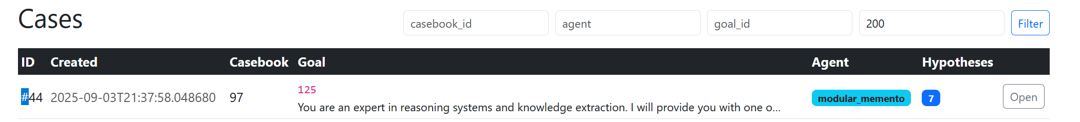
Caption:
🗂️ The Casebook in SIS each card represents a case, with its reasoning outputs, scores, and metadata. The Casebook is where Stephanie’s past experiences are stored, organized, and continually refined ready to be retrieved for the next reasoning challenge.
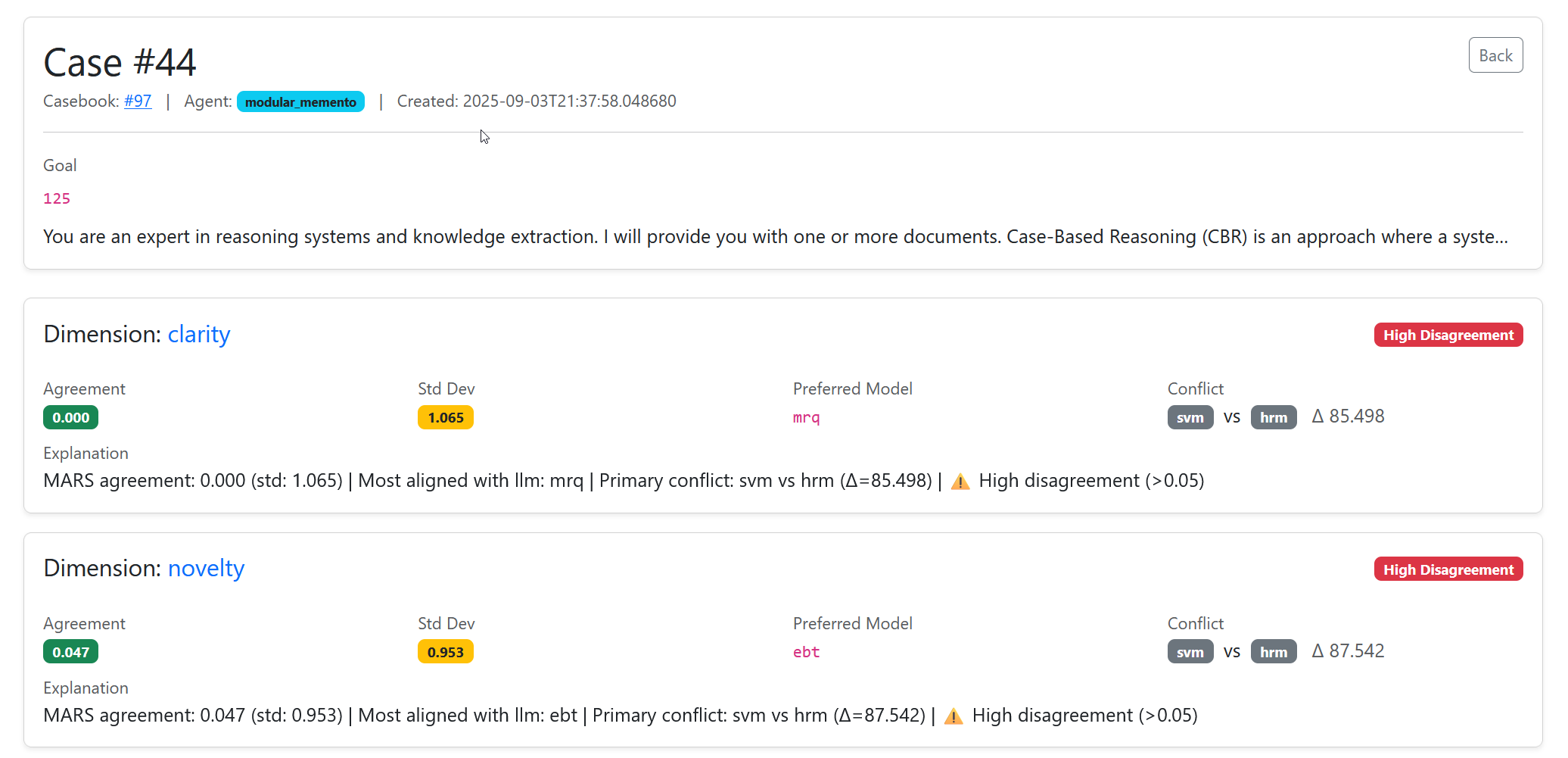
🗂️ An example Case in SIS Here you can see some of the detaisl of an actual case.
    flowchart TD
    subgraph Casebook["📚 Casebook (SIS)"]
        C1[📝 Case 1<br/>Reasoning Trace + Scores]
        C2[📝 Case 2<br/>Reasoning Trace + Scores]
        C3[📝 Case 3<br/>Reasoning Trace + Scores]
    end

    A[🎯 New Goal] --> B[🔍 Retrieve Relevant Cases]
    B --> C1 & C2
    C1 & C2 --> D[♻️ Reuse + Adapt Reasoning]
    D --> E[🛠️ Revise with Feedback]
    E --> F[💾 Retain Updated Case]
    F --> Casebook

    style Casebook fill:#f9f,stroke:#333,stroke-width:2px
    style A fill:#bbf,stroke:#333,stroke-width:2px
    style F fill:#cfc,stroke:#333,stroke-width:2px
After all these moving parts, you might be wondering: why does this matter? Isn’t this just another layer of complexity on top of Stephanie’s pipelines?
💡 This is where the shift happens.
The CBR middleware isn’t just an implementation detail it’s the point where intelligence decouples from model size. While most AI progress chases larger models, Stephanie gets smarter through better algorithms specifically, through the CBR loop.
💡 Why This Changes Everything
Stephanie’s implementation achieves something profound: it decouples intelligence from model size. While most AI progress comes from bigger models, Stephanie gets smarter through better algorithms specifically, through the CBR loop.
This means:
- ✅ Stephanie can run on smaller, cheaper models while still improving
- ✅ Her knowledge base grows independently of model capacity
- ✅ She can transfer learning across completely different domains
As the Memento paper hints: “The policy is continually updated based on environmental feedback through a memory rewriting mechanism.” Stephanie makes this concrete with measurable outcomes.
This isn’t just “better AI” it’s a fundamental shift toward algorithms over parameters, where intelligence lives in the reasoning process itself.
📋 Memento: Checklist of Implementation
The entire purpose of this post was to bring the Memento paper off the page and into a working system. Here’s the checklist what the paper proposed, and how we built it inside Stephanie:
| Memento (Paper) | Stephanie (Implementation) | ✅ |
|---|---|---|
Reasoning traces as cases – record (state, plan, reward) |
PlanTraces – structured records with goals, inputs, steps, outputs, errors, and scores | ✅ |
| Case bank – store past cases for later retrieval | PlanTrace Store (Postgres/SQLite) – database-backed memory with embeddings, metadata, and APIs | ✅ |
| Case retrieval by similarity (KNN) | Embedding Store (H-Net, HF, Ollama) – vector search over traces, documents, and hypotheses | ✅ |
| Adaptation over generation – reuse past cases instead of starting from scratch | PlannerReuseAgent – ranks and adapts top traces into new plans via LLM prompting | ✅ |
| Feedback and revision – correct and refine cases with signals | Multi-dimensional scoring (HRM, SICQL, MRQ, EBT, SVM) – graded evaluation of reasoning and documents | ✅ |
| Retention policies – decide what to keep, prune, or discard | RetentionPolicy module – configurable rules (keep_all, keep_top_k, discard_failed) |
✅ |
| Champion selection – prioritize strong past cases | ChampionPromoter + GoalStateTracker – mark and promote best cases per goal | ✅ |
| AB validation – compare case variants | ABValidator – runs controlled comparisons across candidate solutions | ✅ |
| Learning loop – improve without fine-tuning models | MicroLearner – online updates that adapt ranking and scoring based on past performance | ✅ |
| (Optional in paper) Q-retriever for quality-weighted retrieval | ScorableRanker + MARS – composite scoring and meta-analysis of scorer agreement | ✅ |
🛑 Conclusion
We started with a question: can an AI learn from its own experience without constant fine-tuning?
The Memento paper gave us the blueprint: intelligence can live in a memory of cases. In this post, we turned that blueprint into a working, extensible system inside Stephanie.
Here’s what we built:
- 🧩 CBR Middleware Layer – a reusable class that can wrap any pipeline, not just a single agent.
- 📊 Scorable Abstraction – a universal way to make every concept (documents, traces, rules) measurable and comparable.
- ⚖️ Multi-Dimensional Judgment – a jury of scorers (HRM, SICQL, MARS) that evaluate reasoning beyond simple rewards.
- 🌐 Memory Graph – not just logs, but a connected lineage of reasoning, with explicit reuse links across PlanTraces.
This isn’t just an implementation. It’s a foundation. With this CBR loop in place, Stephanie can now improve every time she acts by remembering, reusing, and revising her own reasoning.
👉 What’s next? In the next post, we’ll connect this living memory to ZeroModel, turning decisions into real-time visual maps. For the first time, you’ll be able to literally watch an AI think.
📖 Glossary
| Term | Definition |
|---|---|
| Stephanie | A self-improving AI system that learns by remembering, reusing, revising, and retaining its reasoning, instead of relying only on fine-tuning. |
| Memento (Paper) | Research paper “Fine-tuning LLM Agents without Fine-tuning LLMs” that proposes case-based reasoning (CBR) as a way for agents to learn from experience. |
| Case-Based Reasoning (CBR) | A cycle of Retrieve → Reuse → Revise → Retain where past reasoning cases are stored, adapted, and improved for new problems. |
| PlanTrace | Stephanie’s structured memory of a reasoning process, containing steps, inputs/outputs, and scores; the atomic “case” in her memory. |
| CBR Middleware | A modular layer in Stephanie that wraps any pipeline with case-based reasoning capabilities (case storage, retrieval, ranking, validation, and retention). |
| Scorable | A universal wrapper that makes any object (document, plan, hypothesis, rule) measurable and comparable by embeddings and scores. |
| ScorableRanker | Component that ranks cases by combining similarity, value, recency, adaptability, and diversity into a weighted score. |
| MARS (Model Agreement & Reasoning Signal) | A meta-analysis tool that checks if scorers agree, detects conflicts, and identifies the most reliable evaluator. |
| HRM (Hierarchical Reasoning Model) | A model that simulates layered reasoning by alternating between high-level strategies and low-level steps, producing a judgment with reasoning trace. |
| SICQL (Scalable In-Context Q-Learning) | A model with Q, V, and π heads that scores quality, value, and action policies directly over embeddings for sharp evaluation. |
| Retention Policy | Rules that decide which cases to keep or discard (e.g., keep all, keep top-K, discard failed) to ensure memory grows in quality. |
| Casebook | A structured collection of related PlanTraces and reasoning cases grouped by goal, domain, or experiment. |
| ContextNamespacer | Middleware module that tags each case with goal/run IDs to prevent scope collisions in memory. |
| CasebookScopeManager | Decides which casebooks to search or update when storing and retrieving cases. |
| CaseSelector | Retrieves candidate past cases for reuse, balancing champions, recent successes, novelty, and exploration. |
| Quality Assessor | Filters out low-quality cases before they are added to casebooks, ensuring only useful cases are retained. |
| Champion Promoter | Elevates the best-performing case to “champion” status for a given goal, making it the default for reuse. |
| AB Validator | Runs A/B testing between candidate cases to validate which one performs better in practice. |
| MicroLearner | Lightweight reinforcement loop that fine-tunes scorers and retrieval weights using feedback from case performance. |
| ZeroModel | A complementary system that visualizes Stephanie’s decision-making process through Visual Policy Maps, enabling real-time introspection of reasoning. |
📚 References
Further Reading / Tools
-
Stephanie Insight System (SIS)
Dashboard for exploring cases, traces, and scorers in Stephanie. Makes CBR pipelines visible and debuggable. GitHub Repo -
ZeroModel & Visual Policy Maps
Complementary system for compressing high-dimensional policy data into images, allowing “AI you can watch think.” See blog post: Visual Policy Maps on zeromodel.org. -
Case-Based Reasoning (Classic AI)
A. Aamodt & E. Plaza (1994)
“Case-Based Reasoning: Foundational Issues, Methodological Variations, and System Approaches”.
The foundational survey that first systematized CBR in AI. -
Unstructured.io
Python library used for PDF parsing in Stephanie’sDocumentProfilerAgent. Docs -
arXiv API
Stephanie’s entry point for retrieving new knowledge cases. Docs
📎 Appendix: 📥 retrieve
🔎 Step 1: Retrieve The ArxivSearchAgent
The first step in Case-Based Reasoning (CBR) is always retrieval. In the Memento paper, this means pulling similar cases from memory. In Stephanie, we extend this to include not just internal memory but also external knowledge sources starting with scientific papers from arXiv.
Why arXiv? Because Stephanie is designed for self-learning research workflows. To improve over time, she needs a steady flow of new problems, methods, and evidence. ArXiv is the natural place to start: it’s where cutting-edge research lives.
🛠️ The Agent: ArxivSearchAgent
👉 I Full Code Here
We’ve covered this agent before (see DeepResearch Part 1 📄), but here’s a quick recap of how it works:
-
Keyword extraction – It takes the current goal text and extracts candidate keywords using simple heuristics (later stages refine them).
-
Query building – Constructs an arXiv-compatible search query, filtering by year, category (
cs.AIby default), and optionally by recency (today, week, month, year). -
Fetching results – Uses the
arxivPython API, with retry logic for empty page errors. – Each result is normalized into a structured dict:title,summary,url,authors,category, etc. -
Context integration – Results are stored back into the pipeline context so downstream agents can use them for profiling, scoring, and planning.
📖 Remembering Everything
As we’ve said before, Stephanie is a pipeline application. Everything she does big or small, nested or top-level is a pipeline. And more than that: every pipeline is a PlanTrace. That means every run, every stage, every output becomes a learning moment, a piece of memory that can be retrieved, reused, revised, or retained.
Here’s how it looks in practice:
    flowchart TD
    %% Style
    classDef pipeline fill:#f6f8fa,stroke:#0366d6,stroke-width:2px,color:#000
    classDef step fill:#fff5e6,stroke:#f59e0b,stroke-width:2px,color:#000
    classDef memory fill:#e6fffa,stroke:#10b981,stroke-width:2px,color:#000
    classDef index fill:#eef2ff,stroke:#6366f1,stroke-width:2px,color:#000

    %% Pipeline (top row)
    subgraph P["⚙️ Pipeline Execution"]
      A[🔍 Arxiv Search]
      B[📄 Document Loader]
      C[🧩 Profiler]
      D[📊 Paper Scorer]
      E[♻️ Planner Reuse]
      F[📝 Knowledge Loader]
      G[📦 Cartridge Retain]
    end
    class P pipeline

    %% Execution steps (middle row)
    subgraph S["🪢 Execution Steps (PlanTrace)"]
      H1[Arxiv Search Step]
      H2[Doc Loader Step]
      H3[Profiler Step]
      H4[Paper Score Step]
      H5[Planner Reuse Step]
      H6[Knowledge Loader Step]
      H7[Cartridge Retain Step]
    end
    class S step

    %% Memory + Indexing (bottom row)
    subgraph M["🧠 Memory + Indexing"]
      I[🔎 Embedded & Indexed]
      J[♻️ Reuse Links + Retrieval]
    end
    class M memory

    %% Connections
    A --> H1 --> I
    B --> H2 --> I
    C --> H3 --> I
    D --> H4 --> I
    E --> H5 --> I
    F --> H6 --> I
    G --> H7 --> I
    I --> J --> E
This layering Pipeline → PlanTrace → Memory ensures that every action Stephanie takes is both execution and learning. By embedding, indexing, and linking traces back into memory, Stephanie turns pipelines into a feedback system where experience itself becomes training data.
🚀 Let’s do some science
In this post by starting with arXiv retrieval, we:
- Anchor Stephanie’s reasoning in real, high-quality scientific work.
- Generate cases worth remembering.
- Ensure that the Retrieve step isn’t abstract it’s directly tied to solving real research goals.
  stages:
     - name: arxiv_search
       agent_role: retrieve
       description: "📥 Retrieve: search Arxiv for candidate documents (knowledge cases)"
       cls: stephanie.agents.knowledge.arxiv_search.ArxivSearchAgent
       enabled: true
       iterations: 1
✅ Next, we’ll walk through what happens after retrieval how papers become structured intelligence, scored, and eventually reused.
📥 Step 2: Materialize The DocumentLoaderAgent
Please note we covered this in more detail in this post.
Now that we’ve retrieved candidate papers from arXiv, the next step is to materialize them into structured, scorable knowledge objects.
This is where the DocumentLoaderAgent comes in.
It doesn’t just “download a PDF” it transforms a raw document into a first-class citizen of Stephanie’s memory:
- ✅ Downloads and extracts text
- ✅ Stores in Postgres
- ✅ Generates H-Net embeddings
- ✅ Assigns domains (NLP, ML, Robotics, etc.)
- ✅ Links to the current pipeline run
- ✅ Logs every action
This is not ingestion it’s assimilation.
🛠️ The Agent: DocumentLoaderAgent
Let’s walk through the key parts of the code that make this possible.
1. Skip Duplicates, Store New
# Skip if already exists
existing = self.memory.documents.get_by_url(url)
if existing:
    stored_documents.append(existing.to_dict())
    continue
- Prevents redundant processing
- Ensures idempotency the same paper won’t be loaded twice
2. Download & Extract PDF
response = requests.get(url, stream=True)
# ... write to temp file ...
text = PDFConverter.pdf_to_text(pdf_path)
os.remove(pdf_path)
- Uses
requests+PDFConverterto extract clean text - Handles streaming for large files
- Cleans up temp files
3. Create a Scorable
scorable = Scorable(
    id=doc_id,
    text=embed_text,
    target_type=TargetType.DOCUMENT,
)
self.memory.scorable_embeddings.get_or_create(scorable)
🔍 New Concept: What’s a
Scorable?
A Scorable is the atomic unit of memory in Stephanie.
Every object that can be retrieved, scored, or reused documents, plan traces, hypotheses must be a Scorable.
This guarantees that it has:
- ✅ An embedding (via H-Net)
- ✅ A type (
document,plan_trace,hypothesis) - ✅ A text field for retrieval
- ✅ A score bundle (HRM, SICQL, MRQ, etc.)
By making everything a Scorable, we ensure that no knowledge is unindexed.
4. Generate Embeddings with H-Net
embed_text = f"{doc['title']}\n\n{doc.get('text', doc.get('summary', ''))}"
- Combines title + full text (or summary) for rich context
- Passed to
H-Netviaget_or_create()→ stored inembeddingstable
👁️ New Concept: Embeddings as “Vision”
Think of H-Net as Stephanie’s eyes.
Just as your brain converts light into neural signals, H-Net converts text into dense vectors that represent meaning.
Once embedded, documents can be:
- 🔍 Searched by similarity
- 🗺️ Mapped in a vector space
- 🔄 Retrieved for reuse
This is how Stephanie “sees” knowledge.
5. Assign Domains with ScorableClassifier
results = self.domain_classifier.classify(
    text, self.top_k_domains, self.min_classification_score
)
for domain, score in results:
    self.memory.scorable_domains.insert({
        "scorable_id": str(document.id),
        "scorable_type": "document",
        "domain": domain,
        "score": score,
    })
📂 New Concept: Domains as Categories
A document isn’t just “about AI” it might be:
- 80% NLP
- 15% Optimization
- 5% Ethics
The DomainClassifier assigns multiple overlapping domains with confidence scores.
This lets Stephanie:
- 🔎 Filter by domain (
"show me all NLP papers") - 🎯 Weight retrieval by relevance
- 🧠 Build domain-specific skill clusters
6. Link to Pipeline Run
self.memory.pipeline_references.insert({
    "pipeline_run_id": pipeline_run_id,
    "target_type": TargetType.DOCUMENT,
    "target_id": doc_id,
    "relation_type": "inserted",
    "source": self.name,
})
- Creates a provenance link between the document and the pipeline
- Enables traceability: “Which run loaded this paper?”
- Supports retention policies: “Keep all docs from high-quality runs”
🧩 The Full Ingestion Flow
    flowchart TD
    A[📥 Search Result] --> B{Already in DB?}
    B -->|Yes| C[🔁 Link to Run]
    B -->|No| D[⬇️ Download PDF]
    D --> E[📄 Extract Text]
    E --> F["🧠 Generate Embedding<br/>(H-Net)"]
    F --> G["🏷️ Assign Domains<br/>(NLP, ML, etc.)"]
    G --> H[💾 Store Document]
    H --> I[🔗 Link to Pipeline]
    I --> J[🪢 PlanTrace Updated]

    subgraph "Memory Layer"
        F --> K[Embeddings Table]
        G --> L[Domains Table]
        H --> M[Documents Table]
        I --> N[Pipeline References]
    end

    J --> O[✅ Ready for Profiling]
🚀 An information machine
The DocumentLoaderAgent is where external knowledge becomes internal memory.
It enforces a critical invariant:
Every piece of knowledge must be scorable, embeddable, classifiable, and linkable.
This is what makes CBR possible:
- ✅ You can retrieve documents by similarity
- ✅ You can reuse them in planning
- ✅ You can revise them with feedback
- ✅ You can retain them in a structured way
Without this agent, you’d just have PDFs.
With it, you have a living growing knowledge base.
👀 Viewing Imported Documents in SIS
One of the challenges in building these pipelines is that so much of the work happens “under the hood.” With SIS (Stephanie Insight System), we make this process visible.
Every document that DocumentLoaderAgent processes is immediately available to explore inside SIS:
- 📋 List View – See all documents loaded by a pipeline run, with ID, title, summary, source, and scorable metadata.
- 🔍 Detail View – Click into a document to see its full text, assigned domains, embedding info, and provenance links back to the pipeline run.
📋 Document List
Figure showing SIS document list view. Each row represents a scorable document: title, summary, and source are shown. From here you can click through to inspect details.
🔍 Document Details
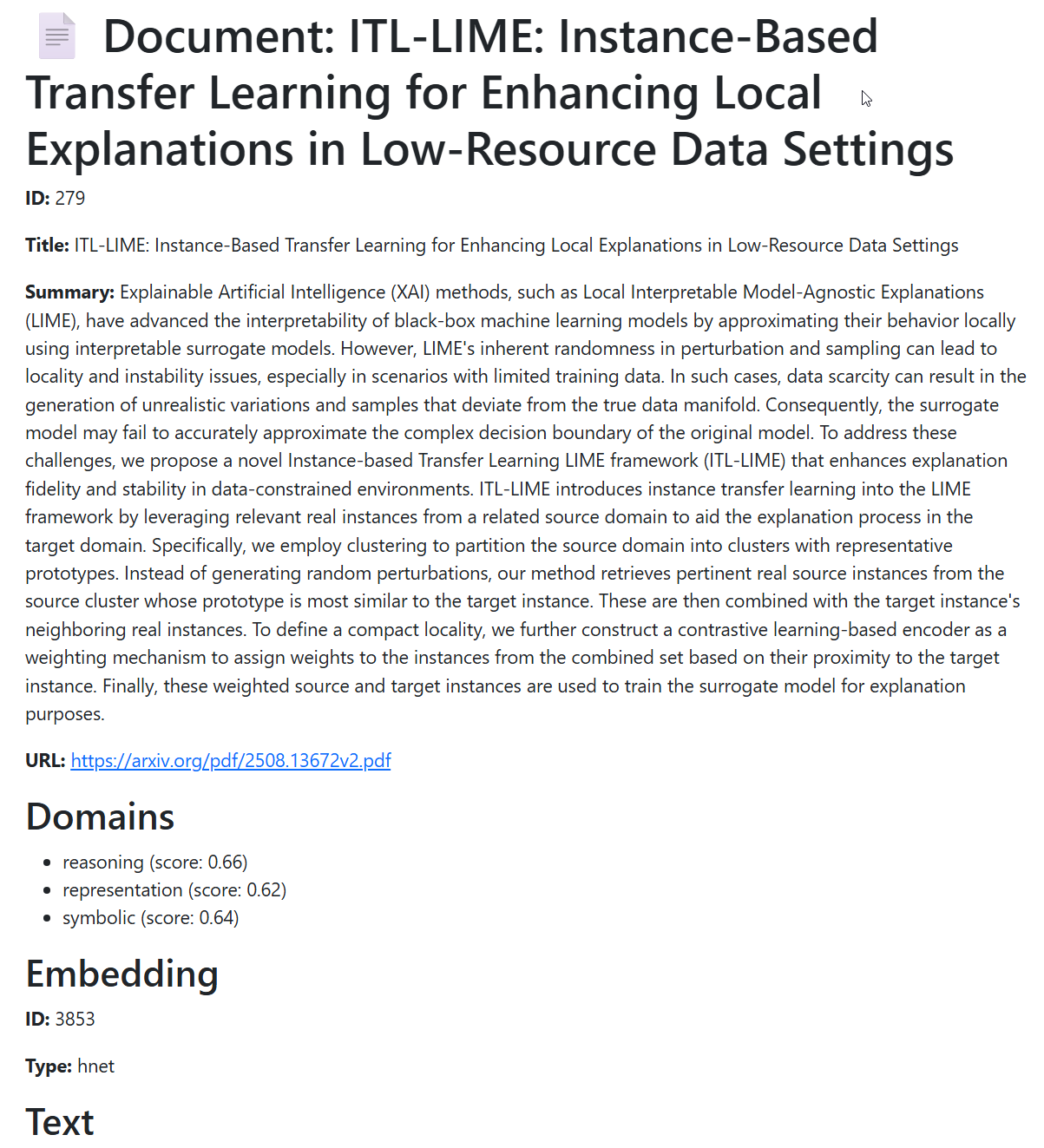
Figure showing the SIS document detail page. On the detail page you see everything the system knows about this document full text, embeddings, assigned domains, and how it links back into the pipeline run. This makes the “invisible ingestion” pipeline completely transparent.
🌐 Easy visual inspection of the process
This is more than a UI convenience. By making imported documents explorable in SIS, we:
- ✅ Verify that ingestion worked (no silent failures).
- ✅ Inspect assigned domains and embeddings.
- ✅ Trace provenance from document → scorable → pipeline run.
- ✅ Build trust: you can see exactly what knowledge Stephanie has taken in.
👉 This closes the loop between code (the agent) and cognition (Stephanie’s growing memory).
📌 Next Step: Profile
Now that we’ve loaded the documents, the next stage is profiling breaking them into structured sections (abstract, method, results) so they can be reused effectively.
🧱 Step 3: Structure The DocumentProfilerAgent
Now that we’ve retrieved papers and loaded them into memory, the next challenge is: how do we make them usable?
A PDF is not a plan. A title and abstract are not a case.
To use a document in Case-Based Reasoning (CBR), we need to break it down into structured sections abstract, methods, results, contributions so we can:
- 🔍 Retrieve by section (“find papers with strong ablation studies”)
- 🧠 Reuse specific parts of reasoning
- 📊 Score each component independently
- 🔄 Revise and refine over time
This is the job of the DocumentProfilerAgent.
It doesn’t just “read” a paper it dissects it, classifies its parts, and prepares it for reuse.
🛠️ The Agent: DocumentProfilerAgent
1. Unstructured Parsing: The First Attempt
unstruct_data = self.section_parser.parse(text)
- Uses
unstructured.io(or similar) to extract sections via layout analysis - Works well on modern PDFs with clean formatting
- Fast, deterministic, no LLM cost
But as you know real-world documents are messy:
- Headers misaligned
- Sections merged or missing
- Equations, figures, and footnotes corrupt the flow
So while unstructured parsing is fast, it’s not reliable enough on its own.
2. Fallback to LLM: The Temptation (and Trap)
if self.fallback_to_llm and self.needs_fallback(unstruct_data):
    llm_data = await self.extract_with_prompt(text, context)
We could use an LLM to:
- Read the full text
- Output a clean JSON with
abstract,methods, etc.
But in practice, this didn’t work well. ❌ Quality Drift – Summaries were often shallow, missing key technical details.
So while LLMs seem like a solution, they introduced more noise than signal.
3. The Right Answer: Trust the Source
Instead of generating summaries, we decided to trust the authors.
✅ arXiv provides a summary using their API.
Why?
- It’s written by experts
- It’s concise and accurate
- It’s already available from the
arxiv_searchstage
This is a key insight:
Don’t re-summarize what’s already well-summarized.
So the DocumentProfilerAgent:
- ✅ Keeps the original abstract
- ✅ Uses it as the
summaryfield - ✅ Only falls back to LLM if truly missing
This ensures quality, consistency, and efficiency.
4. Merge & Validate: Best of Both Worlds
chosen = self.merge_outputs(unstruct_data, llm_data)
When fallback is needed, we don’t just pick the LLM version we compare quality.
The merge_outputs method:
- Checks length
- Evaluates content quality (sentence coherence, word complexity)
- Picks the best version, not just the longest
def evaluate_content_quality(self, text: str) -> float:
    sentences = text.split(".")
    avg_word_len = sum(len(word) for word in text.split()) / len(text.split())
    sentence_score = len([s for s in sentences if len(s.strip()) > 20]) / max(1, len(sentences))
    return 0.4 * min(1.0, len(text)/500) + 0.4 * sentence_score + 0.2 * min(1.0, avg_word_len/8)
This heuristic scorer acts as a gatekeeper, ensuring only high-quality content enters memory.
🏷️ The Domain Classifier: Categorizing Knowledge
Once sections are extracted, the next step is classification.
section_domains = self.domain_classifier.classify(text, top_k=3, min_score=0.6)
🔍 New Concept: What’s a
Domain? ADomainis a category of knowledge likeNLP,Computer Vision,Ethics, orRobotics.
But unlike a single label, the DomainClassifier assigns multiple domains with confidence scores:
[
  {"domain": "NLP", "score": 0.85},
  {"domain": "Reasoning", "score": 0.72},
  {"domain": "Efficiency", "score": 0.61}
]
This lets Stephanie:
- 🔎 Filter by domain: “Show me all reasoning papers”
- 🎯 Weight retrieval: “Prioritize high-NLP papers”
- 🧠 Build domain-specific skills: a
reasoning_agentthat only uses high-scoring reasoning traces
The DomainClassifier is trained on seed examples (in config/domain/seeds.yaml) and uses few-shot classification to generalize.
📌 Note: At this stage, embeddings are still whole-document (title + text). Section-level embeddings will come later, enabling even finer retrieval like “find all method sections in robotics papers.”
🧩 The Full Profiling Flow
    flowchart TD
    A[📄 Raw PDF Text] --> B{Use Unstructured?}
    B -->|Yes| C["🔍 Parse Sections<br/>(abstract, methods, etc.)"]
    B -->|No| D["🧠 LLM Extraction (fallback)"]
    C --> E{Meets Quality?}
    D --> E
    E -->|No| F[🔁 Merge & Score]
    E -->|Yes| G[✅ Accept]
    F --> G
    G --> H[🏷️ Assign Domains]
    H --> I[💾 Store in DB]
    I --> J[🪢 Promote Sections to Scorables]

    subgraph "Memory Layer"
        H --> K[DocumentSectionDomains]
        I --> L[DocumentSection Table]
        J --> M[Embeddings + Scores]
    end
🚀 Tuning information
The DocumentProfilerAgent is where raw information becomes structured intelligence.
It enforces a critical principle:
Don’t generate when you can extract. Don’t guess when you can classify.
By combining:
- ✅ Unstructured parsing (fast, deterministic)
- ✅ arXiv abstracts (trusted, high-quality)
- ✅ Domain classification (multi-label, scored)
- ✅ Quality heuristics (no blind LLM trust)
You’ve built a robust, scalable, and reliable way to turn papers into reusable cases.
In SIS, you’ll soon be able to browse these profiled documents directly titles, abstracts, and assigned domains side by side.
This is what makes CBR possible:
- ✅ You can retrieve by section + domain
- ✅ You can reuse the
methodsof a past paper - ✅ You can revise a plan using high-scoring
results - ✅ You can retain the best knowledge
And most importantly:
This discipline is what makes self-improvement possible: Stephanie builds on what’s real, not what’s imagined.
👀 Seeing the Structure in SIS
It’s one thing to parse and classify a paper into sections it’s another to see it come alive.
That’s where SIS (Stephanie Insight System) steps in. Every profiled document can now be explored through an interactive profile view:
- 📑 Each section (
Abstract,Method,Results, etc.) is shown in its own tab - 🏷️ Domains are highlighted as badges on top of each section
- 📝 Summaries (when available) sit alongside the raw section text
- 🔗 The full provenance (which run loaded this paper, where it came from) is preserved
Here’s what it looks like in SIS:
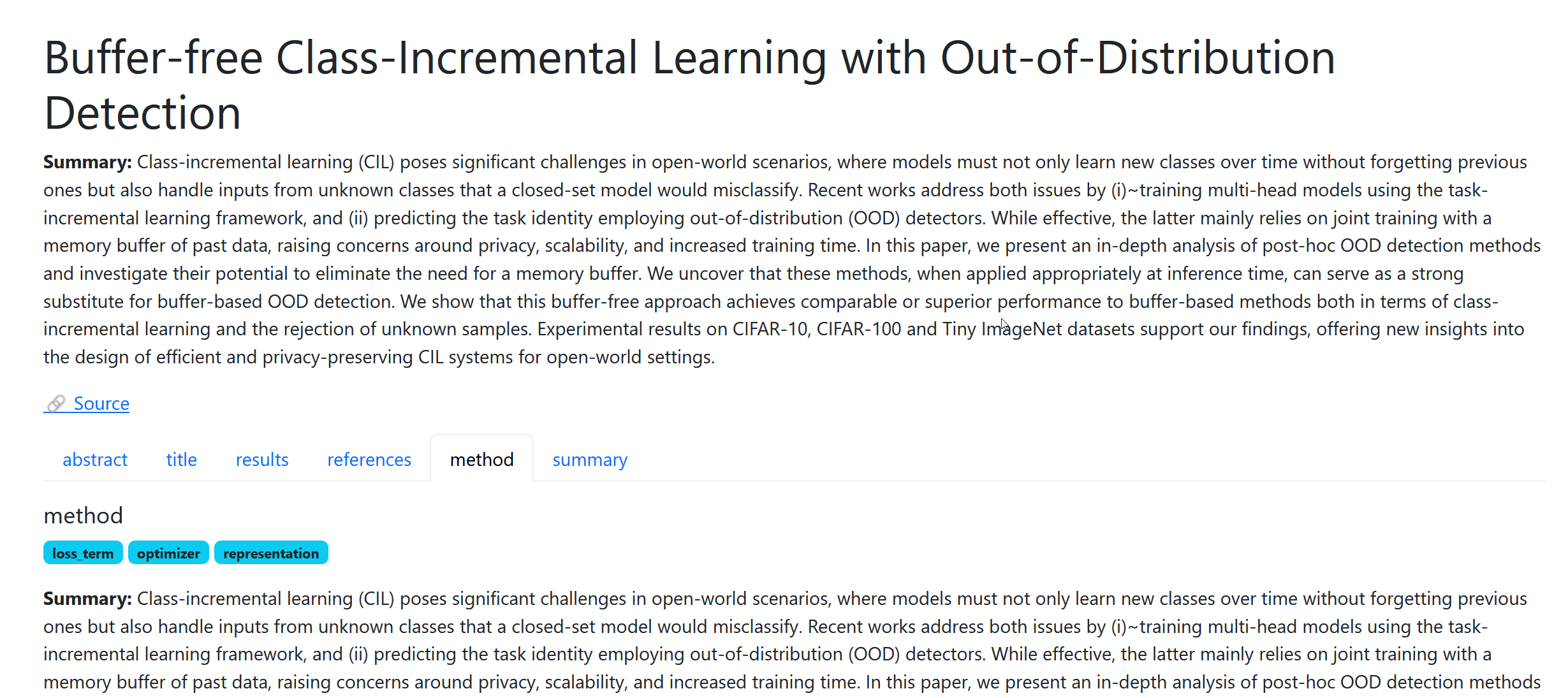
Figure Document Profile in SIS. Notice the tabs per section and the domains attached to each section
With this, a paper stops being a flat PDF and becomes a scored, embeddable, retrievable knowledge object one Stephanie can actually reason over.
🧪 Step 4: Evaluate The PaperScoreAgent and the Multi-Dimensional Judgment of Knowledge
Now that we’ve retrieved, loaded, and structured research papers, the next step is to judge their quality.
Not just “is this paper on-topic?” but:
- Is it novel?
- Is it clear?
- Can we implement its ideas?
- Does it align with our goal?
This is the job of the PaperScoreAgent.
It doesn’t apply a single score it orchestrates a jury of specialized scorers:
- ✅ MRQ → measures relevance
- ✅ SICQL → evaluates clarity & reasoning
- ✅ EBT → scores evidence quality
- ✅ SVM → detects duplication
- ✅ HRM → judges epistemic quality
- ✅ Contrastive Ranker → compares papers relative to each other
Together, they form a multi-dimensional scoring ensemble a cognitive jury that evaluates each paper from multiple angles.
⚖️ Multi-Dimensional Judgment
self.dimensions = [
    "novelty",
    "clarity",
    "relevance",
    "implementability",
    "alignment"
]
These dimensions become decision axes:
- Relevance → does this help the current goal?
- Clarity → can we follow it without guessing?
- Implementability → can we turn it into code or a plan?
- Novelty → is it new, or already solved elsewhere?
- Alignment → does it move us toward our long-term vision?
This is not binary success/failure it’s graded, structured judgment.
2. Ensemble of Scorers
self.scorers = {
    "mrq": MRQScorer(...),
    "sicql": SICQLScorer(...),
    "ebt": EBTScorer(...),
    "hrm": HRMScorer(...),
    "svm": SVMScorer(...),
    "contrastive_ranker": ContrastiveRankerScorer(...)
}
Each scorer contributes to one or more dimensions:
| Scorer | Dimensions It Scores |
|---|---|
| MRQ | Relevance |
| SICQL | Clarity, Reasoning |
| EBT | Evidence, Support |
| HRM | Epistemic Quality, Truth-tracking |
| SVM | Novelty, Duplication |
| Contrastive Ranker | Relative Quality, Preference |
This ensemble approach ensures that no single scorer dominates and that weaknesses I put you down literally but I got to put you down aroundin one are compensated by others.
🧩 From Scores to Meta-Scores (MARS)
After scoring, Stephanie applies MARS the Multi-dimensional Analysis of Reasoning and Scoring.
MARS isn’t a scorer. It’s a meta-analyzer that:
- Aggregates across all papers
- Detects scoring bias (e.g. one scorer is too harsh)
- Identifies high-leverage papers (novel and implementable)
- Recommends which scorers to trust more next time
This is how Stephanie learns to score better over time not just the papers, but the judges themselves.
🧩 The Full Scoring Flow
    flowchart TD
    A[📄 Structured Paper] --> B{Apply Scorers}
    B --> C[MRQ: Relevance]
    B --> D[SICQL: Clarity]
    B --> E[EBT: Evidence]
    B --> F[HRM: Epistemic Quality]
    B --> G[SVM: Novelty]
    B --> H[Contrastive: Preference]

    C --> I[ScoreBundle]
    D --> I
    E --> I
    F --> I
    G --> I
    H --> I

    I --> J[MARS Analysis]
    J --> K[Ranked, Weighted, Trusted Scores]
    K --> L[🪢 PlanTrace Updated]

    subgraph "Memory Layer"
        I --> M[ScoreBundle Table]
        K --> N[MARS Recommendations]
    end
🚀 Why This Matters for CBR
In Case-Based Reasoning, cases are only useful if they’re good cases.
The PaperScoreAgent ensures that:
- ✅ High-quality cases rise to the top
- ✅ Retrieval ranks by multi-dimensional quality, not just similarity
- ✅ Stephanie continuously refines its own judges
Without it, CBR would be garbage in, garbage out. With it, Stephanie builds a curated library of strong, reusable cases.
🧠 Step 5: Judge The HRM Scorer and the Quality of Reasoning
But there’s a deeper question than “is the paper good?”:
Was the reasoning itself good?
Not “did it get the right answer?” but “was the thinking behind it sound?”
This is where the Hierarchical Reasoning Model (HRM) comes in. HRM doesn’t just score knowledge it thinks about thinking.
🔍 Two Flavors of HRM
HRMScorer→ scores(goal, document)pairs: is this paper well-reasoned?EpistemicPlanHRMScorer→ scoresPlanTraces: was this reasoning process itself good?
This dual design means Stephanie can judge both:
- The knowledge she consumes (documents)
- The reasoning she performs (traces)
⚙️ How HRM Thinks
HRM is built as a hierarchical loop of cognition:
- 🔹 Low-Level RNN (L) → models fine-grained reasoning steps
- 🔹 High-Level RNN (H) → models strategic updates over time
Together, they simulate multi-step thinking and produce an epistemic quality score.
    flowchart TD
    A[Input: Goal + Trace] --> B[Embed & Encode]
    B --> C[Low-Level RNN: step-by-step]
    B --> D[High-Level RNN: strategy updates]
    C --> E[zL_final]
    D --> F[zH_final]
    E & F --> G["Epistemic<br/>Quality Score (0–1)"]
Why this matters:
- ✅ Rewards structured, coherent reasoning
- ✅ Penalizes shallow pattern-matching
- ✅ Exposes introspectable states (
zL,zH) → a window into the “shape” of thought
📊 Why HRM Fits CBR
Traditional CBR says: reuse any past case that worked. But brittle success can hide bad reasoning.
HRM flips this:
Only reuse cases with high-quality reasoning.
That makes CBR self-correcting: Stephanie learns not just from results, but from good thinking itself.
🚀 Why HRM is Critical for Self-Improvement
- Policy Learning (GILD): HRM scores train planning policies on good reasoning.
- MCTS Guidance: HRM scores act as a compass when exploring.
- Retention: Bad reasoning traces are pruned, even if they had “right” answers.
- Skill Acquisition: New skills are learned only from high-HRM traces.
♻️ Step 6: Reuse The PlannerReuseAgent and Learning from the Past
Now that Stephanie can judge knowledge (PaperScoreAgent) and judge reasoning (HRM), the next step is to reuse the best cases.
This is the job of the PlannerReuseAgent.
It works like this:
- Retrieve → find past PlanTraces most similar to the current goal
- Filter → select only those with high HRM scores
- Adapt → use LLMs to reshape past plans into a new solution
- Link → record parent-child reuse links, so lineage is never lost
    flowchart LR
    A[🎯 Current Goal] --> B[Retrieve Past PlanTraces]
    B --> C[Filter: High HRM Quality]
    C --> D[Adapt with LLM]
    D --> E[New Plan Trace]
    E --> F[🔗 Record Reuse Link]
This closes the CBR loop:
- Retrieve → good past cases
- Reuse → adapt them to new goals
- Revise → update with feedback
- Retain → store as new cases for the future
♻️ Step 6: Reuse The PlannerReuseAgent and the Memory Graph
Now that we’ve retrieved, structured, and scored past reasoning traces, the next step is reuse.
This is where Case-Based Reasoning (CBR) becomes real: Stephanie doesn’t generate a plan from scratch she adapts one from her own history.
This is the job of the PlannerReuseAgent.
It’s not just a planner it’s a reasoning archaeologist, digging through past PlanTraces to find the best strategies for the current task.
🛠️ The Agent: PlannerReuseAgent
Let’s walk through how it works and why it’s more than just “RAG for plans”.
1. Retrieve Candidate Traces
all_traces = self.memory.plan_traces.get_all(limit=500)
- Fetches up to 500 past
PlanTraces - Converts each into a
Scorable(for embedding)
🔍 Why This Matters
EveryPlanTraceis treated as a first-class knowledge object embeddable, scoreable, reusable.
2. Embed & Rank with ScorableRanker
ranked = self.ranker.rank(query=query_scorable, candidates=candidates, context=context)
The ScorableRanker computes a composite score using four signals:
| Signal | Purpose | Formula |
|---|---|---|
| Similarity | Semantic match to current goal | cosine_sim(goal_emb, trace_emb) |
| Reward | Did the trace succeed? | avg_score from EvaluationORM |
| Recency | Penalize outdated traces | exp(-age_sec / (30*24*60*60)) |
| Adaptability | Has this trace been reused successfully? | reuse_count / attempt_count |
rank_score = sum(components[k] * self.weights.get(k, 0) for k in components)
✅ Weighted Combo
Default:similarity=0.4, reward=0.3, recency=0.2, adaptability=0.1
Configurable per task or domain
This is not just retrieval it’s value estimation.
3. Adapt Top Traces into a New Plan
prompt = self.prompt_loader.load_prompt(self.cfg, context)
response = self.call_llm(prompt, context=merged)
parsed = self._extract_plan_from_response(response)
The LLM is given:
- The current goal
- The top-K ranked traces (goal, plan, rank_score)
And asked to adapt them into a new plan.
The prompt includes:
## Rationale: Why these cases?
## Score: 8/10
## Plan:
1. Search for relevant papers
2. Extract key claims
3. Compare with current goal
This ensures the new plan is not a copy, but a synthesis.
4. Record Reuse Links
self.memory.plan_traces.add_reuse_link(
    parent_trace_id=parent_trace_id,
    child_trace_id=new_trace_id
)
This is critical.
It creates a directed link from the new trace (child) to the past traces (parents) that inspired it.
These links form a memory graph a lineage of reasoning that shows how knowledge evolves.
🧩 The Reuse Flow
    flowchart TD
    A[🎯 Current Goal] --> B[📚 All PlanTraces]
    B --> C[🧠 Embed with H-Net]
    C --> D[📊 Rank: Similarity + Reward + Recency + Adaptability]
    D --> E[🔝 Top-K Traces]
    E --> F[🔄 LLM Adapts into New Plan]
    F --> G[🔗 Record Reuse Links]
    G --> H[🪢 PlanTrace Updated]

    subgraph "Memory Layer"
        D --> I[ScorableRanker Weights]
        G --> J[Reuse Links Table]
        H --> K[PlanTrace Store]
    end
🌐 The Memory Graph
Every reuse link turns your PlanTrace store into a graph of reasoning evolution.
    graph TD
    A[Trace 1: Summarize Memento] --> B[Trace 2: Explain Memento]
    B --> C[Trace 3: Compare Memento vs RAG]
    C --> D[Trace 4: Implement CBR in Stephanie]
    D --> E[Trace 5: Optimize VPM Retrieval]
This is not just logging it’s knowledge lineage.
You can:
- 🔍 Find all traces derived from a breakthrough idea
- 📈 Measure how reasoning quality improves over generations
- 🛠️ Debug failures by tracing back to root causes
🚀 Why This Closes the CBR Loop
The PlannerReuseAgent is where memory becomes intelligence.
It ensures that:
- ✅ Only high-quality, recent, adaptable traces are reused
- ✅ New plans are synthesized, not copied
- ✅ The provenance of every decision is recorded
- ✅ The memory graph grows with every task
This is not just reuse it’s self-improvement.
🧠 Step 6: The PlanTraceMonitor Memento’s Case Bank in Action
Now that we’ve seen how Stephanie retrieves, structures, scores, and reuses knowledge, we need to look at the core infrastructure that makes it all possible: the PlanTraceMonitor.
This isn’t just a logger.
It’s Memento’s Case Bank brought to life.
📄 What Memento Says
In the paper, the Case Bank is where all reasoning episodes are stored:
“Each case is a (state, plan, reward) tuple, stored for later retrieval and reuse.”
It’s the memory of the agent the foundation of self-improvement.
But the paper leaves implementation open.
We’ve filled that gap and gone further.
🛠️ Key Features of the PlanTraceMonitor
1. Automatic Trace Creation
def start_pipeline(self, context: Dict, pipeline_run_id: str):
    self.current_plan_trace = PlanTrace(
        trace_id=str(pipeline_run_id),
        goal_text=context.get("goal", {}).get("goal_text", ""),
        plan_signature=self._generate_plan_signature(context),
        input_data=self._extract_input_data(context),
        execution_steps=[],
        meta={ "started_at": time.time() }
    )
- Every pipeline run becomes a
PlanTrace - No manual logging it’s automatic, universal, and consistent
2. Step-by-Step Monitoring
def start_stage(self, stage_name: str, context: Dict, stage_idx: int):
    step = ExecutionStep(
        step_id=f"{trace_id}_step_{stage_idx + 1}",
        step_type=stage_name,
        input_text=input_preview,
        output_text="",
        start_time=time.time()
    )
    self.current_plan_trace.execution_steps.append(step)
- Every stage is logged as an
ExecutionStep - Duration, errors, and outputs are captured
3. Scorable-Aware Output Capture
def complete_stage(self, stage_name: str, context: Dict, stage_idx: int):
    agent_obj = context.get("agent_obj")
    if agent_obj and getattr(agent_obj, "is_scorable", False):
        details = getattr(agent_obj, "scorable_details", {})
        step.input_text = details.get("input_text", "")
        step.output_text = details.get("output_text", "")
- Only agents that are truly scorable (LLM, reasoning, summarization) populate
input_text/output_text - Others get a breadcrumb (context keys), not a fake output
- This ensures only meaningful steps are scored
4. Scoring & Feedback Loop
async def score_pipeline(self, context: Dict):
    scoring_context = {
        "plan_traces": [self.current_plan_trace],
        "goal": context.get("goal", {})
    }
    scored_context = await self.plan_trace_scorer.run(scoring_context)

    self.current_plan_trace.pipeline_score = scored_context.get("pipeline_score", {})
    self.current_plan_trace.mars_analysis = scored_context.get("mars_analysis", {})
- Uses HRM, SICQL, MRQ, EBT to assign epistemic quality
- Enables value estimation for future retrieval
5. Retention Policies
def apply_retention_policy(self):
    if self.retention_policy == "discard_failed":
        failed = self.memory.plan_traces.get_failed()
        for t in failed:
            self.memory.plan_traces.delete(t.trace_id)
keep_all: grow foreverkeep_top_k: retain only the bestdiscard_failed: prune the useless
This ensures the memory grows in quality, not just quantity.
6. Reuse Links (Memory Graph)
def link_reuse(self, parent_trace_id: str, child_trace_id: str):
    self.memory.plan_traces.add_reuse_link(parent_trace_id, child_trace_id)
- Every time a new plan adapts from a past trace, a directed link is recorded
- This creates a memory graph a lineage of reasoning
    graph TD
    A[Trace 1: Summarize Paper] --> B[Trace 2: Explain Method]
    B --> C[Trace 3: Compare to Memento]
    C --> D[Trace 4: Implement CBR]
This is not just logging it’s knowledge evolution.