Real Problems. AI Solutions.

How We Used AI to Analyze When U.S. Debt Becomes a Constraint
Executive Summary
We demonstrate a human + AI research process.
AI was used to:
- refine the question
- identify the correct metric
- expose assumptions
- and test the model through adversarial critique
The goal was to transform a vague macro concern into a quantifiable, testable system model.
The Question
We began with a simple but vague concern:
“Is U.S. debt becoming a problem?”
Through iterative analysis, this was refined into:
“When does interest on U.S. debt become a constraint on the system?”
Key Finding
The critical variable is:
Interest as a percentage of federal revenue
At present:
- Federal revenue ≈ $5.6 trillion
- Net interest ≈ $1.0 trillion
Which implies:
Interest already consumes ~18–19% of federal revenue
What Happens Next
Under different assumptions:
-
Baseline scenario: ~25% threshold reached in the mid-2030s
-
Higher-for-longer rates: threshold reached around 2030–2031
-
Stress scenario: threshold reached around 2029
When refinancing dynamics are included:
These timelines move forward by approximately 1–2 years
What This Means
This does not imply collapse.
It implies a structural shift:
An increasing share of government resources is consumed by past obligations
Leading to:
- reduced fiscal flexibility
- increased trade-offs
- greater sensitivity to shocks
Why the Method Matters
The most important outcome of this work is not the numbers.
It is the method.
AI was used not to produce conclusions — but to systematically improve the quality of reasoning.
By forcing:
- clearer questions
- explicit assumptions
- model validation
- and adversarial testing
The process reduces the risk of:
- hidden bias
- weak reasoning
- or untested conclusions
Final Insight
Debt becomes a problem when it grows faster than the system that supports it.
Understanding that relationship and testing it rigorously is the core contribution of this analysis.
1. Introduction: The Problem & The Confusion
Over the past few years, one number has started to dominate discussions about the U.S. economy:
Interest on the national debt.
It is now approaching $1 trillion per year, and depending on who you ask, this means one of two things:
- The system is on the brink of collapse
- Or everything is completely under control
Both views are confident. Neither is particularly precise.
That’s the problem.
Most discussions around debt focus on scale, not structure. We hear large numbers trillions, deficits, projections but very little clarity on what actually matters inside the system.
Is $1 trillion dangerous? Does it need to become $2 trillion or $3 trillion before it matters? Or is the real signal something else entirely?
At the same time, this problem is not isolated.
Interest rates are no longer near zero. Demographic growth across the West is slowing. Geopolitical tensions are increasing uncertainty in energy markets and capital flows.
These are not independent variables. They interact.
Which makes the core issue harder:
This is not a single-variable problem. It is a system.
And systems are where intuition tends to fail.
A Different Approach
Instead of starting with a conclusion, this post does something different.
We treat AI not as an answer engine, but as a reasoning partner.
The goal is not to predict collapse, or to argue that everything is fine.
The goal is much more specific:
At what point does interest on the U.S. debt become a meaningful constraint on the system?
To answer that, we don’t jump straight to conclusions.
We:
- break the problem down
- challenge assumptions
- build a simple model
- and stress test the results
This post is both:
- an analysis of U.S. debt dynamics
- and a demonstration of how to use AI to reason about complex problems
2. Why Use AI for This Problem
Macroeconomic systems are difficult to reason about for a simple reason:
They are nonlinear, multi-variable, and full of hidden assumptions.
Humans are good at intuition in simple environments. We are not as good when:
- multiple variables interact
- feedback loops exist
- small assumption changes produce large outcome shifts
This is exactly the type of problem we’re dealing with.
**Example AI Prompt:**

--"What assumptions in this model are most likely to fail under higher interest rates?"--

**Key Output:**
- refinancing lag underestimated
- growth assumptions optimistic
- rate persistence risk underweighted
Where Human Reasoning Breaks Down
Take a simple example:
“Interest is $1 trillion that sounds bad.”
That statement feels meaningful, but it’s incomplete.
It ignores:
- how large the economy is
- how fast revenue is growing
- what interest rates are doing
- how debt is structured
Without those, the number alone doesn’t tell you much.
This is where most discussions stall:
- strong opinions
- weak models
What AI Is Actually Good At
AI is not useful here because it “knows the answer.”
It’s useful because it can:
- reframe questions
- surface hidden assumptions
- iterate quickly across scenarios
- challenge its own reasoning when prompted correctly
In other words:
AI helps move from intuition → structure
What AI Is Bad At
To use AI properly, we also need to be clear about its limitations.
AI will:
- sound confident even when wrong
- rely heavily on input framing
- default to consensus assumptions
- occasionally hallucinate details
So we cannot treat it as an authority.
Instead:
We treat AI as a tool that must be audited.
The Right Mental Model
The most useful way to think about AI in this context is:
Not as a predictor but as a structured thinking system.
We don’t ask:
- “What will happen?”
We ask:
- “What are the variables?”
- “What assumptions are we making?”
- “What happens if those assumptions are wrong?”
That shift is what makes the analysis meaningful.
3. The AI Research Framework
To make this concrete, we used a simple but powerful framework.
This is the part you can reuse not just for debt, but for any complex system.
Step 1 Decompose the Problem
We start with a vague question:
“Is U.S. debt becoming a problem?”
This is too broad.
So we break it down into components:
- total debt
- interest payments
- government revenue
- interest rates
- economic growth
- demographics
This step matters because:
You cannot analyze what you have not separated.
Step 2 Identify the Right Metric
Initially, the instinct is to focus on:
- total debt
- or total interest
AI helps challenge this.
Through iteration, we arrive at a better metric:
Interest as a percentage of government revenue
Why this matters:
- it measures burden, not size
- it scales with the system
- it reflects real constraints
This is the first major shift:
From big number thinking → ratio thinking
Step 3 Extract Assumptions
Once the metric is defined, the next step is to make assumptions explicit.
Every model depends on assumptions, whether stated or not.
Key assumptions include:
- interest rates remain stable or decline
- economic growth continues at a steady pace
- population supports labor force expansion
- government revenue grows with GDP
Most analyses stop here and accept these implicitly.
We do the opposite.
Step 4 Stress the Assumptions
This is where the analysis becomes meaningful.
We actively challenge each assumption:
Interest Rates
- Were the last 15 years artificially low?
- What if rates settle structurally higher?
Growth
- What if GDP growth is overstated?
- What if productivity slows?
Demographics
- What happens if population growth weakens?
- What if immigration declines?
Each of these pushes the system in the same direction:
Interest grows faster relative to revenue
Step 5 Build a Simple Model
Instead of building a complex model, we intentionally keep it simple.
We define:
- interest growth rate
- revenue growth rate
And track how the ratio evolves over time.
This allows us to answer a precise question:
“When does the burden cross a meaningful threshold?”
Step 6 Generate Scenarios
We then test multiple cases:
- baseline (official projections)
- higher interest rates
- weaker growth
- combined stress scenario
The goal is not to predict one future.
The goal is to understand:
How sensitive the system is to changes in assumptions
Step 7 Adversarial Validation
This is the most important step and the one most people skip.
We explicitly ask:
- Where could this be wrong?
- Which assumptions are weakest?
- What evidence contradicts this?
We use AI to critique its own reasoning.
This is how we avoid:
- false confidence
- one-sided narratives
- hidden bias
Step 8 Synthesis
Only after all of that do we form conclusions.
Not absolute claims, but structured insights:
- what matters most
- what drives outcomes
- where the risks are
Figure 1: The AI-Assisted Research Process for Complex Systems
Before applying the model, it is useful to understand the process used to construct it.
Figure 1 illustrates the structured workflow used throughout this analysis. Rather than asking AI for answers, we use it to progressively refine the problem, expose assumptions, and stress test the model.
This process transforms an initially vague question into a structured, testable system.
    flowchart TD
    A["🤔 Start with a vague problem"]
    B["🔧 Decompose the system"]
    C["🎯 Identify the correct metric"]
    D["📋 Extract assumptions explicitly"]
    E["⚠️ Stress test assumptions"]
    F["🏗️ Build a simple transparent model"]
    G["📊 Run baseline and stress scenarios"]
    H["🛡️ Adversarial validation"]
    I["🔄 Refine model and assumptions"]
    J["🧠 Synthesize conclusions"]
    K["📚 Document limits, sources, calculations"]

    E1["💰 Rates"]
    E2["📈 Growth"]
    E3["👥 Demographics"]
    E4["🔄 Refinancing"]
    E5["🌍 External shocks"]

    H1["❓ What could be wrong?"]
    H2["🔍 Which assumptions are weakest?"]
    H3["📉 What evidence contradicts this?"]

    A --> B --> C --> D --> E --> F --> G --> H --> I --> J --> K

    E --> E1
    E --> E2
    E --> E3
    E --> E4
    E --> E5

    H --> H1
    H --> H2
    H --> H3

    style A fill:#d4e6f1,stroke:#2980b9,stroke-width:2px
    style B fill:#d4e6f1,stroke:#2980b9,stroke-width:2px
    style C fill:#d4e6f1,stroke:#2980b9,stroke-width:2px
    style D fill:#d4e6f1,stroke:#2980b9,stroke-width:2px
    style E fill:#fdebd0,stroke:#e67e22,stroke-width:2px
    style F fill:#d4e6f1,stroke:#2980b9,stroke-width:2px
    style G fill:#d4e6f1,stroke:#2980b9,stroke-width:2px
    style H fill:#e8f5e9,stroke:#2e7d32,stroke-width:2px
    style I fill:#d4e6f1,stroke:#2980b9,stroke-width:2px
    style J fill:#d4e6f1,stroke:#2980b9,stroke-width:2px
    style K fill:#d5f5e3,stroke:#27ae60,stroke-width:2px

    style E1 fill:#fff3e0,stroke:#e67e22,stroke-width:1px
    style E2 fill:#fff3e0,stroke:#e67e22,stroke-width:1px
    style E3 fill:#fff3e0,stroke:#e67e22,stroke-width:1px
    style E4 fill:#fff3e0,stroke:#e67e22,stroke-width:1px
    style E5 fill:#fff3e0,stroke:#e67e22,stroke-width:1px

    style H1 fill:#e8f5e9,stroke:#2e7d32,stroke-width:1px
    style H2 fill:#e8f5e9,stroke:#2e7d32,stroke-width:1px
    style H3 fill:#e8f5e9,stroke:#2e7d32,stroke-width:1px
Figure 1. AI-assisted research workflow. The process moves from problem definition to decomposition, metric selection, assumption extraction, stress testing, modeling, scenario analysis, and adversarial validation. The key feature is iteration: each stage feeds back into refinement, improving the quality of the final conclusions.
The Key Idea
The framework can be summarized simply:
AI is used to refine the problem until the answer becomes clear.
Not by guessing.
But by systematically:
- breaking down
- testing
- and validating
Transition to the Analysis
Now that the framework is defined, we can apply it.
The next step is to take this process and use it to answer a concrete question:
At what point does interest on U.S. debt become a constraint on the system?
4. Applying the Framework: U.S. Debt as a System
With the framework established, we now apply it to a concrete case:
When does interest on U.S. debt become a constraint on the system?
4.1 The Initial Question
Public discourse typically starts here:
“Interest is approaching $1 trillion per year is that sustainable?”
At first glance, this appears to be the right question.
But using the AI framework, we immediately challenge it.
This question focuses on scale, not structure.
And in a system as large as the U.S. economy, scale alone is misleading.
4.2 AI Reframing
Through iterative reasoning, the question evolves into something more precise:
From:
“How large will interest become?”
To:
“At what point does interest constrain the system?”
This reframing is critical.
Because what matters is not how large a number becomes in isolation, but how it behaves relative to the system that supports it.
4.3 Identifying the Correct Metric
Applying the framework, we test several candidates:
- Total debt → too abstract
- Total interest → lacks context
- Debt-to-GDP → slow-moving, indirect
We converge on:
Interest as a percentage of federal revenue
This metric captures:
- the burden of past obligations
- the share of resources consumed
- the remaining fiscal flexibility
It turns a vague concern into a measurable constraint.
4.4 Current Position
Using official data:
- Federal revenue (2026): ~$5.6 trillion
- Net interest (2026): ~$1.0 trillion
This implies:
Interest already consumes ~18–19% of federal revenue
This is not a distant problem.
It is already a meaningful component of the system.
4.5 Defining a Stress Threshold
Rather than defining a hard “crisis point,” we introduce analytical thresholds:
| Range | Interpretation |
|---|---|
| ~20% | Early constraint, reduced flexibility |
| ~25% | Meaningful fiscal pressure |
| ~30%+ | Severe constraint policy trade-offs intensify |
These are not mechanical limits.
They are heuristics used to understand system pressure.
4.6 Why ~25% Matters
The choice of ~25% as a stress threshold is not arbitrary.
At this level:
Approximately one-quarter of all federal revenue is consumed by interest payments.
Mathematical Interpretation: Why 25% Is a Structural Threshold
The significance of ~25% can be understood directly from the budget constraint.
\[ \text{Discretionary Space} = \text{Revenue} - \text{Interest} - \text{Mandatory Spending} \]At an interest burden of 25%:
- 75% of revenue remains after debt service
- Mandatory spending typically absorbs ~60–65% of revenue
- Leaving ~10–15% of total revenue available for all discretionary functions
This creates a compressed fiscal structure in which:
A large share of public resources is pre-committed to past obligations, rather than current policy priorities.
Unlike most spending categories, interest payments do not directly fund public services or investment. They represent the cost of financing prior deficits.
As this share rises, the budget becomes increasingly constrained, and policy choices become more zero-sum.
This threshold is further reinforced by debt dynamics:
$$ \Delta \left(\frac{D}{Y}\right) = (r - g)\frac{D}{Y} - pb $$When \( r > g \), the debt ratio increases unless offset by primary surpluses.
At higher interest burdens, generating those surpluses becomes progressively more difficult, because the fiscal space required to adjust is itself reduced by rising interest costs.
Taken together, these relationships imply that:
Around the 25% level, the system transitions from flexible allocation to constrained allocation.
This is why the threshold is best understood as a tipping point in fiscal flexibility, rather than a point of mechanical failure.
This has three important implications:
1. Budget Constraint
Interest becomes one of the largest expenditure categories, reducing fiscal flexibility and forcing trade-offs between:
- discretionary spending
- taxation
- and additional borrowing
2. Historical Context
While the United States is unique (reserve currency, deep capital markets), the mechanics of fiscal stress are not. Historical episodes show consistent patterns when interest burdens approach or exceed 20-25% of revenue:
| Country / Episode | Interest/Revenue Peak | Outcome |
|---|---|---|
| Italy, 2011-2012 | ~22-24% (IMF data) | Bond yields spiked to 7.4%, triggering ECB intervention and technocratic government |
| UK, 1976 | ~20-25% (estimated) | IMF program, spending cuts, shift in macro policy paradigm |
| Emerging Markets (avg.) | >20% | Associated with debt distress, IMF programs, or restructuring |
| US, Early 1990s | ~14-15% (peak) [[25]] | Bipartisan deficit reduction (1990, 1993), followed by surpluses |
Key observation: No advanced economy has sustained interest burdens above ~25% of revenue for an extended period without either:
- Major fiscal consolidation, or
- Financial repression (keeping rates below inflation), or
- Exceptional growth that outpaced debt accumulation
The United States has not yet reached this threshold—but it is approaching it faster than at any point since the early 1990s.
3. System Sensitivity
At higher burden levels, the system becomes more sensitive to changes in:
- interest rates
- growth assumptions
- refinancing dynamics
Small changes in inputs can produce disproportionately large effects on the budget.
For these reasons, ~25% is used as a practical threshold for meaningful constraint, not as a hard limit or crisis point.
A Warning, Not a Cliff
25% is not a mechanical failure point. The United States will not “run out of money” at this level.
Rather, 25% marks the transition from:
Fiscal flexibility → Fiscal constraint
| Burden Level | Character |
|---|---|
| <20% | Interest is a manageable budget line item |
| 20-25% | Trade-offs become visible; policy debates intensify |
| >25% | Every budget decision is shadowed by debt service; crisis response capacity narrows |
This is why the threshold matters: not as prophecy, but as an early-warning signal that the system is losing slack.
4.7 The Core Insight
This leads to the central idea of the analysis:
The risk is not that interest becomes extremely large.
The risk is that it grows faster than the system that supports it.
This sets up the model.
5. Data, Model & Assumptions
To move from intuition to analysis, we construct a simple, transparent model.
The goal is not precise forecasting.
The goal is:
Clarity, reproducibility, and testability, to understand system behavior under changing assumptions.
5.1 Starting Data
We anchor the model in current conditions:
- Revenue (2026): ~$5.6T
- Net interest (2026): ~$1.0T
- Interest burden: ~18.6% of revenue
These serve as the baseline.
5.2 Model Definition
We define:
$$ S_t = \frac{\text{Interest}_t}{\text{Revenue}_t} $$Assuming:
- interest grows at rate \(g_I\)
- revenue grows at rate \(g_R\)
We derive:
$$ S_t = S_0 \cdot \left(\frac{1 + g_I}{1 + g_R}\right)^t $$This defines a relative growth differential system.
In exact form, the burden evolves according to the ratio:
$$ \frac{1 + g_I}{1 + g_R} $$For modest growth rates, this is approximately governed by the sign of:
\((g_I - g_R)\)
but the ratio form is exact.
This allows us to calculate:
When the system crosses defined stress thresholds
If:
- \(g_I > g_R\) → burden increases exponentially
- \(g_I \approx g_R\) → system evolves slowly (near-stable, path-dependent)
- \(g_I < g_R\) → burden declines
A persistent gap of just 2–3 percentage points between \(g_I\) and \(g_R\) will compound over time, leading to large changes in the burden over a decade.
5.3 Why This Model
We deliberately use a simplified structure.
Because:
- complex models obscure assumptions
- simple models expose them
This model allows:
- easy replication
- clear sensitivity analysis
- transparent critique
5.4 Key Assumptions
Interest Growth \( g_I \)
Driven by:
- total debt expansion
- prevailing interest rates
- refinancing dynamics
Revenue Growth \( g_R \)
Driven by:
- nominal GDP growth
- population and labor force trends
- inflation
5.5 Refinancing A Critical Reality
In practice, interest costs do not adjust instantly.
Only a portion of debt is refinanced each year.
A useful approximation:
- Average maturity ≈ 6 years
- → ~15–20% of debt rolls over annually
This means:
- rate changes affect the system gradually
- not all debt reprices immediately
5.6 Modeling Choice
We consider two approaches:
A. Smooth Growth Model (Primary Model)
- Uses an average growth rate \( g_I \)
- Implicitly captures gradual repricing
B. Refinancing (Rollover) Model
-
Explicitly models:
- maturing debt
- new issuance
- evolving average rate
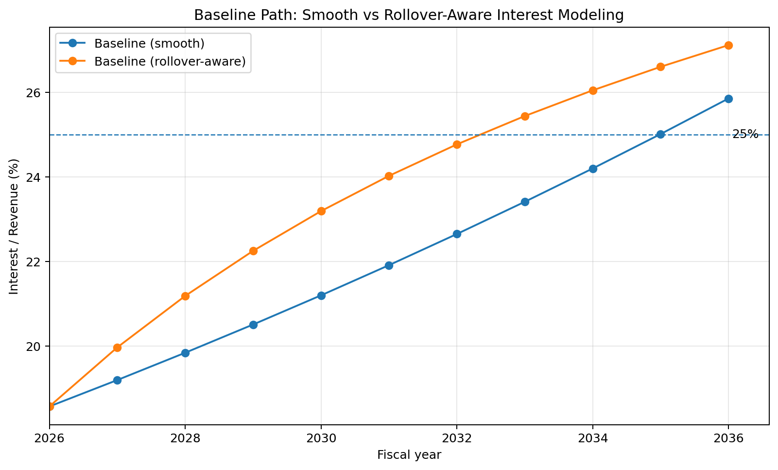
5.7 Validation Through Refinancing
To test robustness, we compare both approaches.
Result:
In a rising-rate environment, refinancing causes interest costs to increase faster in early years
Because:
- new debt is issued at higher rates immediately
- maturing debt rolls over progressively
Empirically:
Interest costs can be 15–25% higher over a 5-year window compared to the smooth model
Figure 2 A refinancing-aware model can push the burden higher earlier than a smooth-growth approximation, because maturing debt and new issuance reprice into a higher-rate environment over time.
5.8 Implication for the Model
This gives us a key insight:
The simplified model is directionally correct but slightly conservative
Meaning:
Real-world dynamics may push the system to stress thresholds earlier
5.9 Final Model Framing
At this point, we have:
- a validated metric
- a transparent model
- explicit assumptions
- a real-world correction layer
We now apply this model across scenarios.
6. Scenario Analysis
The purpose of scenario analysis is not prediction.
It is to understand:
How sensitive the system is to changes in assumptions
6.1 Scenario Design
We define three cases:
| Scenario | Description |
|---|---|
| Baseline | Official projections |
| Higher-for-Longer | Structurally elevated rates |
| Stress Case | High rates + weak growth |
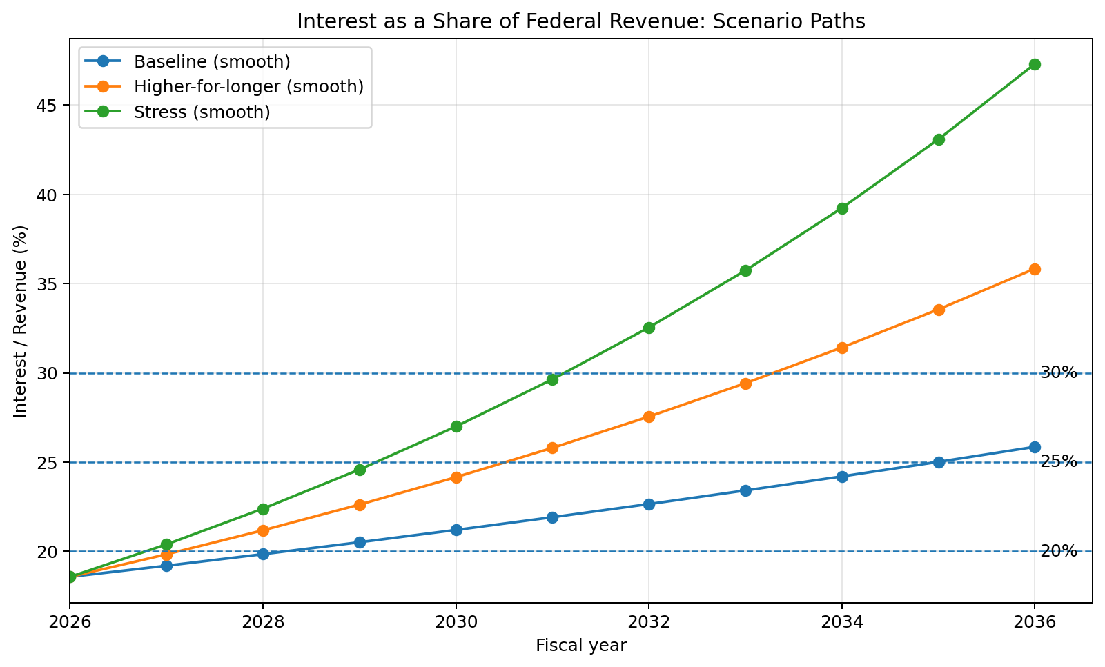
6.2 Baseline Scenario
Assumptions:
- Interest growth: ~7–8%
- Revenue growth: ~4%
Outcome:
The interest burden rises gradually, crossing ~25% in the mid-2030s
This aligns with official projections.
6.3 Higher-for-Longer Scenario
Assumptions:
- Interest growth: ~10%
- Revenue growth: ~3%
Drivers:
- structurally higher interest rates
- slower economic expansion
Outcome:
The system reaches the 25% threshold around 2030–2031
With refinancing effects:
This may shift earlier to ~2028–2030
6.4 Stress Scenario
Assumptions:
- Interest growth: ~12%
- Revenue growth: ~2%
Drivers:
- weak growth
- persistent high rates
- demographic drag
Outcome:
The system reaches the 25% threshold around 2029
With refinancing:
Potentially as early as ~2027–2028
6.5 Comparative Summary
| Scenario | Smooth Model | With Refinancing |
|---|---|---|
| Baseline | ~2035–2036 | ~2033–2034 |
| Higher Rates | ~2030–2031 | ~2028–2030 |
| Stress Case | ~2029 | ~2027–2028 |
Figure 2. Interest as a share of federal revenue under three scenario paths. Starting from the CBO 2026 baseline, the timing of fiscal stress is driven primarily by the gap between interest growth and revenue growth.
6.6 Key Insight
Across all scenarios:
The timeline is highly sensitive to the gap between:
interest growth vs revenue growth
This reinforces the core thesis:
The system does not fail because numbers become large.
It becomes constrained when growth and interest diverge.
For example:
If interest grows at 10% and revenue at 3%:
The burden grows at ~7% relative differential
Over 10 years:
\(S_t ≈ S_0 × (1.07)^10 ≈ ~2×\)
This means:
The burden roughly doubles over a decade
6.7 AI Validation in Practice
This section demonstrates the core strength of the method:
- Initial model → simple, intuitive
- AI critique → identified refinancing gap
- Revised analysis → validated and strengthened
Result:
A model that is:
- transparent
- stress-tested
- and grounded in real-world dynamics
7. Assumption Critique Where the Model Can Break
Up to this point, we have built a model that is:
- transparent
- testable
- and grounded in current data
But the strength of any model is not in its structure.
It is in its assumptions.
The most important question is not whether the model works.
It is whether the assumptions behind it are valid.
This section explicitly challenges those assumptions.
7.1 Interest Rates: A Structural Shift?
The baseline model assumes a relatively stable long-term interest rate environment.
This assumption deserves scrutiny.
Over the past 15 years, interest rates were shaped by:
- post-crisis monetary policy
- quantitative easing
- suppressed term premiums
- global demand for safe assets
This was not a typical regime.
The critical question becomes:
Are we returning to a more “normal” rate environment?
Historically, long-term rates have often been in the 4–6% range.
If that range holds:
- refinancing occurs at higher levels
- average debt cost rises steadily
- interest growth accelerates relative to projections
This does not require a spike.
It only requires:
Rates staying higher than expected for longer
7.2 Growth: Is It Overestimated?
The model assumes moderate nominal growth driven by:
- real economic expansion
- inflation
- labor force growth
Each of these is now under pressure.
Real Growth Constraints
- productivity growth has slowed relative to historical highs
- high debt levels can act as a drag on expansion
- capital allocation may become less efficient in constrained environments
Inflation Uncertainty
- inflation may persist due to structural pressures
- or fall if demand weakens
Both paths create challenges:
- persistent inflation → higher rates
- weak demand → lower revenue growth
7.3 Demographics: The Silent Constraint
Demographics are one of the most underappreciated variables in fiscal analysis.
Across much of the developed world:
- population growth is slowing or declining
- dependency ratios are rising
- labor force expansion is weakening
This directly impacts:
- economic growth
- tax revenue expansion
- long-term fiscal capacity
The United States has historically offset this through immigration.
If that dynamic weakens:
The growth assumptions embedded in the model become less reliable.
7.4 Credit Perception & Feedback Loops
One of the most important dynamics is not directly modeled:
The feedback loop between debt, confidence, and interest rates
As debt grows and interest costs rise:
- investors reassess risk
- term premiums can increase
- borrowing costs rise further
This creates a reinforcing loop:
Debt ↑ → Interest ↑ → Confidence ↓ → Rates ↑ → Interest ↑
For the United States, this does not imply immediate default.
Instead, it implies:
- higher financing costs
- increased volatility
- reduced policy flexibility
7.5 External Pressures
The model also does not explicitly incorporate:
- energy price shocks
- geopolitical fragmentation
- changes in global capital flows
For example:
- sustained high energy prices can increase inflation
- geopolitical risk can raise required returns on capital
- shifts in global reserve behavior can alter demand for government debt
Each of these feeds back into:
Interest rates and growth dynamics
7.6 Summary of Assumption Risk
All major assumptions tend to lean in the same direction:
| Assumption | Risk Direction |
|---|---|
| Interest rates | Higher for longer |
| Growth | Lower than expected |
| Demographics | Structural slowdown |
| Credit perception | Gradual deterioration |
This creates an asymmetric risk profile:
More ways for the system to deteriorate than to improve
8. AI Self-Validation: How the Analysis Was Tested
A central goal of this work is not just analysis, but:
Demonstrating how AI can validate its own reasoning
This section shows how that process worked in practice.
8.1 Initial Errors and Limitations
Early iterations of the analysis contained several weaknesses:
- overemphasis on absolute interest growth
- insufficient focus on relative burden
- implicit acceptance of baseline assumptions
- lack of refinancing realism
These are typical failure modes:
- intuitive but incomplete reasoning
- reliance on familiar narratives
8.2 Iterative Correction
Rather than restating the full framework (Section 3), this section shows how it performed in practice.
8.3 Adversarial Testing
We then used AI in an adversarial role:
- challenge each assumption
- test alternate scenarios
- identify weak points
Examples:
- What if growth is overstated?
- What if rates remain elevated?
- What if refinancing accelerates cost increases?
This step is critical.
Without it:
AI becomes an amplifier of initial bias.
With it:
AI becomes a tool for error detection and refinement.
8.4 Cross-Validation
To ensure robustness:
- model outputs were compared across scenarios
- simplified and more detailed models were aligned
- key results were checked for internal consistency
Notably:
The refinancing model confirmed and slightly accelerated the conclusions of the simpler model
This increases confidence in the result.
8.5 Known Limitations
Despite validation, the model has clear limits:
- it cannot predict policy responses
- it cannot capture sudden shocks
- it is sensitive to input assumptions
- it simplifies complex fiscal dynamics
These limitations are acknowledged explicitly.
8.6 The Role of AI
This process demonstrates the correct role of AI:
Not as a source of truth
But as a system for:
- structuring reasoning
- exposing assumptions
- testing conclusions
9. Interpretation: What This Actually Means
The analysis produces a clear result.
But interpretation requires precision.
9.1 What This Does NOT Mean
This does not imply:
- imminent fiscal collapse
- inability to service debt
- sudden systemic failure
The United States retains:
- monetary sovereignty
- deep capital markets
- structural advantages
9.2 What It DOES Mean
It means:
Interest is becoming an increasing constraint on the system
As the interest burden rises:
- fewer resources remain for discretionary policy
- fiscal flexibility declines
- trade-offs become more severe
This is a constraint dynamic, not a collapse dynamic.
9.3 The Real Risk
The primary risk is not a single event.
It is a gradual shift:
- higher baseline interest costs
- reduced room for policy response
- increased sensitivity to shocks
This makes the system:
More fragile over time
9.4 The Key Variable
Across all scenarios, one variable dominates:
The gap between interest growth and revenue growth
If:
- interest grows faster than revenue → pressure increases
- revenue keeps pace → system stabilizes
Everything else feeds into this relationship.
9.5 Final Insight
The most important conclusion is not a number or date.
It is a framework:
Debt becomes a problem when it grows faster than the system that supports it
And:
AI is valuable not because it predicts the future — but because it helps refine the problem until the structure becomes clear.
10. The General AI Method: A Reusable Framework
This section generalizes the framework described earlier (Section 3).
While this analysis focused on U.S. debt, the real contribution of this work is methodological.
The same approach can be used to analyze any complex system or problem.
What follows is a distilled version of the process used throughout this paper.
10.1 The Core Principle
The key shift is simple:
AI is not used to produce answers. It is used to refine questions until the structure of the problem becomes clear.
10.2 The Eight-Step AI Research Process
Step 1 Define the Problem Clearly
Start with a vague question:
- “Is debt a problem?”
- “Is interest unsustainable?”
Then refine it into something measurable:
“When does interest constrain the system?”
Step 2 Decompose the System
Break the problem into components:
- debt
- interest
- revenue
- rates
- growth
- demographics
This prevents hidden complexity.
Step 3 Identify the Correct Metric
Reject misleading metrics.
Select one that captures system pressure:
Interest / Revenue
This step is often the most important.
Step 4 Extract Assumptions Explicitly
List all assumptions:
- interest rate path
- growth rate
- population trends
- policy stability
Make them visible.
Step 5 Stress Test Assumptions
Challenge each one:
- What if rates are higher?
- What if growth is lower?
- What if demographics worsen?
This prevents model fragility.
Step 6 Build a Simple Model
Prefer:
- clarity
- transparency
- reproducibility
Over complexity.
Step 7 Run Scenarios
Test:
- baseline
- stress
- extreme cases
Focus on sensitivity, not prediction.
Step 8 Adversarial Validation
This is the differentiator.
Use AI to:
- critique the model
- identify weaknesses
- propose alternative explanations
This is where AI shifts from assistant → reviewer.
Figure 4: Applying the AI Framework to U.S. Debt Analysis
While Figure 1 describes the general methodology, Figure 4 shows how this process was applied in practice to the specific case of U.S. debt.
This diagram traces the transformation from an imprecise question to a structured, validated model, highlighting the key decision points and assumption challenges encountered along the way.
    flowchart TD
    Q1["❓ Question: Is US debt becoming a problem?"]
    Q2["🚫 Reject vague framing"]
    Q3["🎯 Reframe: When does interest constrain the system?"]
    Q4["📏 Choose metric: Interest / Revenue"]
    Q5["📊 Collect baseline data"]
    Q6["🏗️ Build simple threshold model"]
    Q7["⚠️ Challenge assumptions"]

    A1["💰 Are rates structurally higher?"]
    A2["📉 Is growth overstated?"]
    A3["👥 Are demographics weakening?"]
    A4["🔄 Does refinancing accelerate pressure?"]

    SCEN1["📈 Run baseline scenario"]
    SCEN2["🔥 Run higher-for-longer scenario"]
    SCEN3["💥 Run stress scenario"]

    COMP["🔁 Compare outputs"]
    REVIEW["🛡️ Adversarial AI review"]
    REVISE["✏️ Revise conclusions"]
    PUBLISH["📚 Publish transparent model, limits, sources"]

    Q1 --> Q2 --> Q3 --> Q4 --> Q5 --> Q6 --> Q7

    Q7 --> A1
    Q7 --> A2
    Q7 --> A3
    Q7 --> A4

    Q7 --> SCEN1
    Q7 --> SCEN2
    Q7 --> SCEN3

    SCEN1 --> COMP
    SCEN2 --> COMP
    SCEN3 --> COMP

    COMP --> REVIEW --> REVISE --> PUBLISH

    style Q1 fill:#d4e6f1,stroke:#2980b9,stroke-width:2px
    style Q2 fill:#fdebd0,stroke:#e67e22,stroke-width:2px
    style Q3 fill:#d4e6f1,stroke:#2980b9,stroke-width:2px
    style Q4 fill:#d4e6f1,stroke:#2980b9,stroke-width:2px
    style Q5 fill:#d4e6f1,stroke:#2980b9,stroke-width:2px
    style Q6 fill:#d4e6f1,stroke:#2980b9,stroke-width:2px
    style Q7 fill:#fdebd0,stroke:#e67e22,stroke-width:2px

    style A1 fill:#fff3e0,stroke:#e67e22,stroke-width:1px
    style A2 fill:#fff3e0,stroke:#e67e22,stroke-width:1px
    style A3 fill:#fff3e0,stroke:#e67e22,stroke-width:1px
    style A4 fill:#fff3e0,stroke:#e67e22,stroke-width:1px

    style SCEN1 fill:#e1f0fa,stroke:#2c7ab1,stroke-width:1px
    style SCEN2 fill:#e1f0fa,stroke:#2c7ab1,stroke-width:1px
    style SCEN3 fill:#e1f0fa,stroke:#2c7ab1,stroke-width:1px

    style COMP fill:#e8f5e9,stroke:#2e7d32,stroke-width:1px
    style REVIEW fill:#e8f5e9,stroke:#2e7d32,stroke-width:1px
    style REVISE fill:#e8f5e9,stroke:#2e7d32,stroke-width:1px
    style PUBLISH fill:#d5f5e3,stroke:#27ae60,stroke-width:2px
Figure 4. Application of the AI research framework to U.S. debt. The process begins with a vague question (“Is debt a problem?”), rejects imprecise framing, and converges on a measurable constraint (Interest / Revenue). Assumptions are then stress tested, scenarios are generated, and results are subjected to adversarial review before final synthesis and publication.
10.3 The Good vs The Bad in AI Analysis
To make this framework practical, we explicitly define:
✅ Good AI Usage
- challenges assumptions
- exposes uncertainty
- produces testable models
- invites critique
❌ Bad AI Usage
- produces confident conclusions without structure
- hides assumptions
- relies on vague narratives
- avoids validation
10.4 Why This Works
This method works because it aligns with how complex systems behave:
- small assumption changes → large outcome differences
- feedback loops dominate outcomes
- linear thinking fails
AI helps by:
forcing structure where intuition would otherwise dominate
10.5 Generalization
This approach is not limited to macroeconomics.
It can be applied to:
- financial markets
- geopolitics
- business strategy
- technology forecasting
Anywhere complexity exists.
11. Conclusion: From Answers to Understanding
This analysis began with a simple question:
“Is U.S. debt becoming a problem?”
It ended with a more precise understanding:
The issue is not the size of the debt.
It is the relationship between interest growth and system capacity.
11.1 What We Learned
- Interest already consumes a significant share of revenue
- The system is sensitive to small changes in assumptions
- Higher rates and weaker growth accelerate stress timelines
- Refinancing dynamics can bring pressure forward
But more importantly:
The system does not fail suddenly.
It becomes constrained gradually.
11.2 The Deeper Insight
The most important conclusion is structural:
Debt becomes a problem when it grows faster than the system that supports it.
Everything else rates, growth, demographics feeds into that relationship.
11.3 The Role of AI
This work also demonstrates something broader.
AI is often framed as:
- a predictor
- an answer engine
- a replacement for expertise
That framing is incomplete.
The real value of AI is:
It enables structured thinking at scale.
It allows us to:
- refine vague questions
- expose hidden assumptions
- test multiple realities
- validate conclusions
11.4 Final Thought
If used incorrectly, AI amplifies noise.
If used correctly, it does something much more powerful:
It reduces complex problems to their essential structure.
And once the structure is clear:
The answer is no longer something you guess.
It is something you derive.
📚 References
Effects of Federal Borrowing on Interest Rates and the Economy
-
Congressional Budget Office. Effects of Federal Borrowing on Interest Rates and the Economy. https://www.cbo.gov/publication/61230
Key finding: Long-run interest rates rise ~2 basis points per 1 ppt increase in debt-to-GDP.
The r-g Differential and Fiscal Sustainability
- Federal Reserve Board. “The r-g Differential and Fiscal Sustainability” (various working papers). https://www.federalreserve.gov/econres/working-papers.htm
When Should Debt Be Reduced?
-
Ostry, J., Ghosh, A., & Espinoza, R. (2015). “When Should Debt Be Reduced?” IMF Staff Discussion Note. https://www.imf.org/en/Publications/Staff-Discussion-Notes
Introduces “fiscal space” as a framework for assessing constraint — aligns with your threshold approach.
Exorbitant Privilege: The Rise and Fall of the Dollar
-
Eichengreen, B. (2011). Exorbitant Privilege: The Rise and Fall of the Dollar. Oxford University Press.
Analyzes how reserve-currency status affects borrowing costs and fiscal flexibility.
Primary Data Sources (Interest Burden / Fiscal Metrics)
-
World Bank. Interest Payments (% of Revenue) – Government Finance Statistics. https://data.worldbank.org/indicator/GC.XPN.INTP.RV.ZS
-
International Monetary Fund. Government Finance Statistics (GFS) Database. https://www.imf.org/en/Data
-
Peter G. Peterson Foundation. Monthly Interest Tracker: U.S. National Debt. https://www.pgpf.org/programs-and-projects/fiscal-policy/monthly-interest-tracker-national-debt
OK* Federal Reserve Economic Data (FRED). Federal Net Interest Payments as % of Federal Receipts (FYOIGDA188S). https://fred.stlouisfed.org/series/FYOIGDA188S
Historical series from 1947–present; useful for contextualizing the 18.6% starting point.
Italy (2011–2012 Eurozone Crisis)
-
European Central Bank. Securities Markets Programme (SMP) and sovereign bond interventions. https://www.ecb.europa.eu
-
International Monetary Fund. Italy: Staff Reports and Article IV Consultations (2010–2013). https://www.imf.org
-
Organisation for Economic Co-operation and Development. Economic Surveys: Italy (2011–2013). https://www.oecd.org
United Kingdom (1976 IMF Crisis)
-
International Monetary Fund. United Kingdom Stand-By Arrangement (1976). https://www.imf.org
-
Bank of England. Historical Monetary and Financial Statistics. https://www.bankofengland.co.uk
-
UK National Archives. The 1976 IMF Crisis and UK Economic Policy Documents. https://www.nationalarchives.gov.uk
Emerging Market Debt Distress (Cross-Country Evidence)
-
International Monetary Fund. Fiscal Monitor Reports (various years). https://www.imf.org/en/Publications/FM
-
World Bank. Global Economic Prospects – Debt and Fiscal Sustainability Chapters. https://www.worldbank.org
-
Reinhart & Rogoff dataset. Historical Sovereign Debt Crises Database.
United States (Early 1990s Fiscal Adjustment)
-
Congressional Budget Office. Historical Budget Data and Economic Outlook Reports. https://www.cbo.gov
-
Office of Management and Budget. Historical Tables, Budget of the U.S. Government. https://www.whitehouse.gov/omb
-
US Treasury. Interest Expense and Debt Data. https://home.treasury.gov
General Sovereign Debt and Fiscal Stress Literature
-
Carmen Reinhart & Kenneth Rogoff. This Time Is Different: Eight Centuries of Financial Folly. Princeton University Press, 2009.
-
International Monetary Fund. Fiscal Sustainability and Debt Dynamics Frameworks.
-
Organisation for Economic Co-operation and Development. Government Debt and Fiscal Sustainability Indicators.
Appendix: Data, Sources, Models, and Validation
This appendix is intentionally comprehensive.
Its purpose is to ensure the analysis is:
- transparent
- reproducible
- auditable
- defensible under scrutiny
A. Data Sources (Primary & Verifiable)
A.1 Fiscal Data
-
Congressional Budget Office Budget and Economic Outlook (2026–2036) https://www.cbo.gov/publication/61882
Key extracted values:
- Revenue (2026): $5.596T
- Net Interest (2026): $1.039T
- Revenue (2036): $8.301T
- Net Interest (2036): $2.144T
-
U.S. Treasury Fiscal Data Portal / Monthly Treasury Statement https://fiscaldata.treasury.gov
Used for:
- validating current interest levels
- validating debt stock
A.2 Interest Rate Data
-
Federal Reserve Economic Data 10-Year Treasury Yield (DGS10) https://fred.stlouisfed.org/series/DGS10
Observations:
- Current range: ~4.2% – 4.5%
- Used as proxy for new issuance rate
A.3 Debt Structure
-
U.S. Treasury Average Maturity of Marketable Debt https://home.treasury.gov
Key assumption:
-
Average maturity ≈ 6 years
-
Implies:
~15–20% of debt refinanced annually
-
A.4 Demographics
-
U.S. Census Bureau https://www.census.gov
-
Congressional Budget Office Used for population, immigration, and labor force trends
B. Core Model Definitions
B.1 Primary Metric
$$ S_t = \frac{\text{Interest}_t}{\text{Revenue}_t} $$Where:
- \(( S_t )\) = interest burden
- Interest = annual net interest payments
- Revenue = federal receipts
B.2 Evolution Formula (Primary Model)
$$ S_t = S_0 \cdot \left(\frac{1 + g_I}{1 + g_R}\right)^t $$Where:
- \(( g_I )\) = interest growth rate
- \(( g_R )\) = revenue growth rate
B.3 Threshold Calculation
$$ t^* = \frac{\ln(\theta / S_0)}{\ln((1 + g_I)/(1 + g_R))} $$Where:
- \(( \theta )\) = threshold (e.g., 25%)
C. Refinancing (Rollover) Model
C.1 Average Rate Evolution
$$ r_{avg,t} = r_{avg,t-1} + (r_{new} - r_{avg,t-1}) \cdot f $$Where:
- \(( f = \frac{1}{\text{maturity}} \approx 0.167 )\)
C.2 Interest Calculation
$$ \text{Interest}_t = \text{Debt}_t \cdot r_{avg,t} $$C.3 Key Insight
Refinancing introduces lagged but accelerating effects:
- Early years → faster-than-expected increases
- Later years → convergence
D. Model Inputs
D.1 Starting Values
| Variable | Value |
|---|---|
| Revenue (2026) | $5.596T |
| Interest (2026) | $1.039T |
| Debt | ~$32T |
| Average rate | ~3.2% |
| Starting ratio | ~18.6% |
D.2 Scenario Parameters
| Scenario | ( g_I ) | ( g_R ) |
|---|---|---|
| Baseline | 7–8% | 4% |
| Higher Rates | 10% | 3% |
| Stress | 12% | 2% |
E. Scenario Results
E.1 Smooth Model Results
| Scenario | Threshold Year (25%) |
|---|---|
| Baseline | ~2035–2036 |
| Higher Rates | ~2030–2031 |
| Stress | ~2029 |
E.2 Refinancing-Adjusted Results
| Scenario | Threshold Year |
|---|---|
| Baseline | ~2033–2034 |
| Higher Rates | ~2028–2030 |
| Stress | ~2027–2028 |
E.3 Interpretation
Refinancing accelerates threshold crossing by approximately 1–2 years
F. Sensitivity Analysis
F.1 Interest Rate Sensitivity
| Change | Effect |
|---|---|
| +1% long-term rates | Material acceleration |
| +2% | Nonlinear increase in burden |
F.2 Growth Sensitivity
| Change | Effect |
|---|---|
| -1% nominal growth | Threshold moves forward |
| -2% | Significant acceleration |
F.3 Combined Effect
Small changes compound:
- Higher rates + lower growth → rapid divergence
G. AI Methodology (Explicit Disclosure)
G.1 How AI Was Used
AI was used to:
- decompose the problem
- identify correct metrics
- extract assumptions
- build and refine models
- perform adversarial critique
G.2 Validation Approach
To ensure robustness:
- assumptions were made explicit
- multiple models were compared
- results were cross-checked
- sensitivity analysis was applied
G.3 Failure Modes Addressed
| Risk | Mitigation |
|---|---|
| Hallucination | Cross-validation |
| Overconfidence | Adversarial prompts |
| Bias | Scenario diversity |
| Oversimplification | Refinancing comparison |
H. Limitations of the Analysis
H.1 Model Limitations
- simplified structure
- does not model full fiscal system
- excludes policy reaction
H.2 Economic Limitations
Cannot predict:
- recessions
- wars
- policy changes
H.3 Structural Assumptions
Assumes:
- continued market access
- stable institutional framework
I. What Would Change the Results
Positive Case
- stronger productivity growth
- higher immigration
- lower long-term rates
Negative Case
- persistent inflation
- geopolitical fragmentation
- reduced demand for Treasuries
J. Reproducibility Guide
J.1 Steps
- Use starting values
- Select \(( g_I )\), \(( g_R )\)
- Apply formula
- compute threshold
J.2 Tools
- spreadsheet
- Python
- calculator
No proprietary tools required.
K. Interpretation Notes
- Thresholds are analytical tools, not hard limits
- Results are directional, not predictive
- Model is assumption-sensitive
L. Final Validation Statement
This analysis is not a prediction model.
It is a structured stress framework designed to:
- identify system pressure
- test assumptions
- evaluate sensitivity
M. Critics Checklist: How to Challenge This Analysis
This section is included to make the analysis fully auditable.
If you disagree with the conclusions, this checklist outlines exactly where and how the analysis can be challenged.
The goal is not to eliminate disagreement.
The goal is to ensure that disagreement is:
precise, structured, and testable
M.1 Challenge the Core Metric
The analysis is built on:
Interest as a percentage of federal revenue
To challenge the conclusions, you must argue that:
- this is not the correct metric, or
- another metric better captures system constraint
Examples of alternative metrics:
- Debt-to-GDP
- Interest-to-GDP
- Primary balance
If a different metric is used:
The full model must be recomputed using that metric.
M.2 Challenge the Starting Data
The baseline depends on:
- Revenue (~$5.6T)
- Interest (~$1.0T)
- Debt (~$32T)
To dispute results, you must provide:
- corrected figures
- or justification for alternative inputs
M.3 Challenge the Growth Assumptions
The model depends on:
- Interest growth rate \(( g_I )\)
- Revenue growth rate \(( g_R )\)
To challenge the conclusions:
- specify alternative values
- justify them with data or reasoning
Examples:
- Lower interest growth (rates fall)
- Higher revenue growth (productivity gains)
M.4 Challenge Interest Rate Assumptions
A key driver of the model is the long-term rate environment.
To challenge:
-
argue that rates will:
- decline structurally
- remain lower than assumed
or
-
provide evidence that:
- term premiums will compress
- global demand will absorb debt
M.5 Challenge the Refinancing Model
The analysis incorporates:
- average maturity (~6 years)
- ~15–20% annual rollover
To dispute:
- provide alternative maturity structure
- argue for different refinancing dynamics
or
-
demonstrate that:
- refinancing effects are overstated
- or incorrectly modeled
M.6 Challenge the Scenario Design
The conclusions rely on three scenarios:
- baseline
- higher-for-longer
- stress
To challenge:
-
propose alternative scenarios
-
demonstrate why:
- rates should be lower
- growth should be stronger
M.7 Challenge the Threshold Definition
The analysis uses:
- 20% → early constraint
- 25% → meaningful pressure
- 30% → severe constraint
To dispute:
-
argue that these thresholds are:
- too low
- too high
- or irrelevant
You must then define an alternative threshold and recompute outcomes.
M.8 Challenge the Structural Assumptions
This analysis assumes:
- continued market access
- stable institutions
- no extreme policy intervention
To challenge:
-
argue that:
- monetary policy will offset stress
- fiscal policy will adjust
- institutional dynamics will change outcomes
M.9 Challenge the Model Itself
The model is intentionally simple.
To challenge:
- propose a more accurate model
- demonstrate how it changes results
However:
The alternative model must remain transparent and reproducible.
M.10 Challenge the Interpretation
Even if the numbers are accepted, interpretation can be challenged.
For example:
- argue that higher interest burden is manageable
- argue that inflation reduces real burden
- argue that reserve currency status offsets risk
M.11 The Standard of Critique
To meaningfully challenge this analysis, a critique must:
- Identify the specific assumption being disputed
- Provide an alternative
- Recompute the outcome
- Compare results
M.12 What Is Not a Valid Critique
The following are insufficient:
- “This won’t happen”
- “The U.S. is different”
- “Markets will adjust”
Without:
- quantified assumptions
- model adjustments
- recalculated outcomes
M.13 Challenge the 25% Threshold
The analysis uses ~25% interest-to-revenue as a practical threshold for meaningful constraint.
This choice is open to challenge.
Potential Critiques
A valid critique may argue:
1. The Threshold Is Too Low
- The system may tolerate higher burdens (e.g. 30–40%)
- Governments can operate under tighter constraints for extended periods
2. Structural Differences (e.g. Japan)
-
Countries such as Japan have sustained:
- higher debt levels
- large central bank ownership of debt
- lower effective interest burdens
This suggests:
The relationship between debt and constraint is institution-specific, not universal
3. Interest Is Not Purely “Lost”
Interest payments are transfers:
- from government → bondholders
- which may include domestic households, institutions, or central banks
This implies:
The economic impact depends on who receives the payments, not just the total level
4. Reserve Currency Effects
The United States benefits from:
- global demand for Treasury assets
- deep capital markets
- dollar reserve status
These factors may:
- reduce refinancing risk
- delay or soften constraint dynamics
5. Inflation as an Adjustment Mechanism
Higher inflation can:
- reduce the real burden of debt
- increase nominal revenue
This may offset rising interest costs in certain scenarios.
Response Within This Framework
This analysis does not claim that:
25% is a universal or deterministic limit
Instead, it uses 25% as a heuristic threshold based on:
- budget structure (compression of discretionary space)
- historical stress patterns (20–25% range)
- system sensitivity (nonlinear response to rate and growth changes)
The key claim is not:
“Constraint occurs exactly at 25%”
But:
Constraint becomes increasingly visible and structurally important in this range
What Would Invalidate the Threshold
To reject the relevance of the 25% threshold, a critique must demonstrate that:
- Higher interest burdens do not materially reduce fiscal flexibility, or
- Structural factors (e.g. monetary policy, demand for debt) fully offset rising interest costs, or
- An alternative threshold better explains when constraint becomes binding
Final Clarification
25% is not a prediction. It is a diagnostic tool.
Its purpose is to:
- identify when the system begins to lose slack
- highlight when trade-offs become unavoidable
- provide a consistent reference point for scenario comparison
M.14 Final Statement
This analysis is not presented as definitive or authoritative.
It is presented as a transparent and testable framework for examining the dynamics of interest, revenue, and fiscal constraint.
If the conclusions are incorrect, it should be possible to identify precisely:
- which assumptions fail
- which inputs are inaccurate
- or where the model structure is insufficient
Conversely, if such failures cannot be clearly demonstrated, it suggests that the underlying structure of the problem may be more robust than initially assumed.
📚 Suggested Citation
Ernan Hughes. (2026). Real Problems. AI Solutions: How We Used AI to Analyze When U.S. Debt Becomes a Constraint.
Available at: https://programmer.ie/post/debt/
Version: 1.0
Date: April 2026
⚖️ License
This document is intended as a working paper and may be updated as new data or assumptions evolve.
This work is licensed under the Creative Commons Attribution-NonCommercial 4.0 International License (CC BY-NC 4.0).
You are free to:
- Share — copy and redistribute the material in any medium or format
- Adapt — remix, transform, and build upon the material
Under the following terms:
- Attribution — You must give appropriate credit
- NonCommercial — You may not use the material for commercial purposes
Full license: https://creativecommons.org/licenses/by-nc/4.0/