We ended the last chapter by changing one number.

rule = 22

became:

rule = 30

Nothing else changed.

Same world.

Same single active cell.

Same three-cell neighborhood.

Same synchronous update.

Same periodic boundary.

Same eight-bit lookup mechanism.

Only the rule changed.

And the spacetime diagram stopped looking simple.

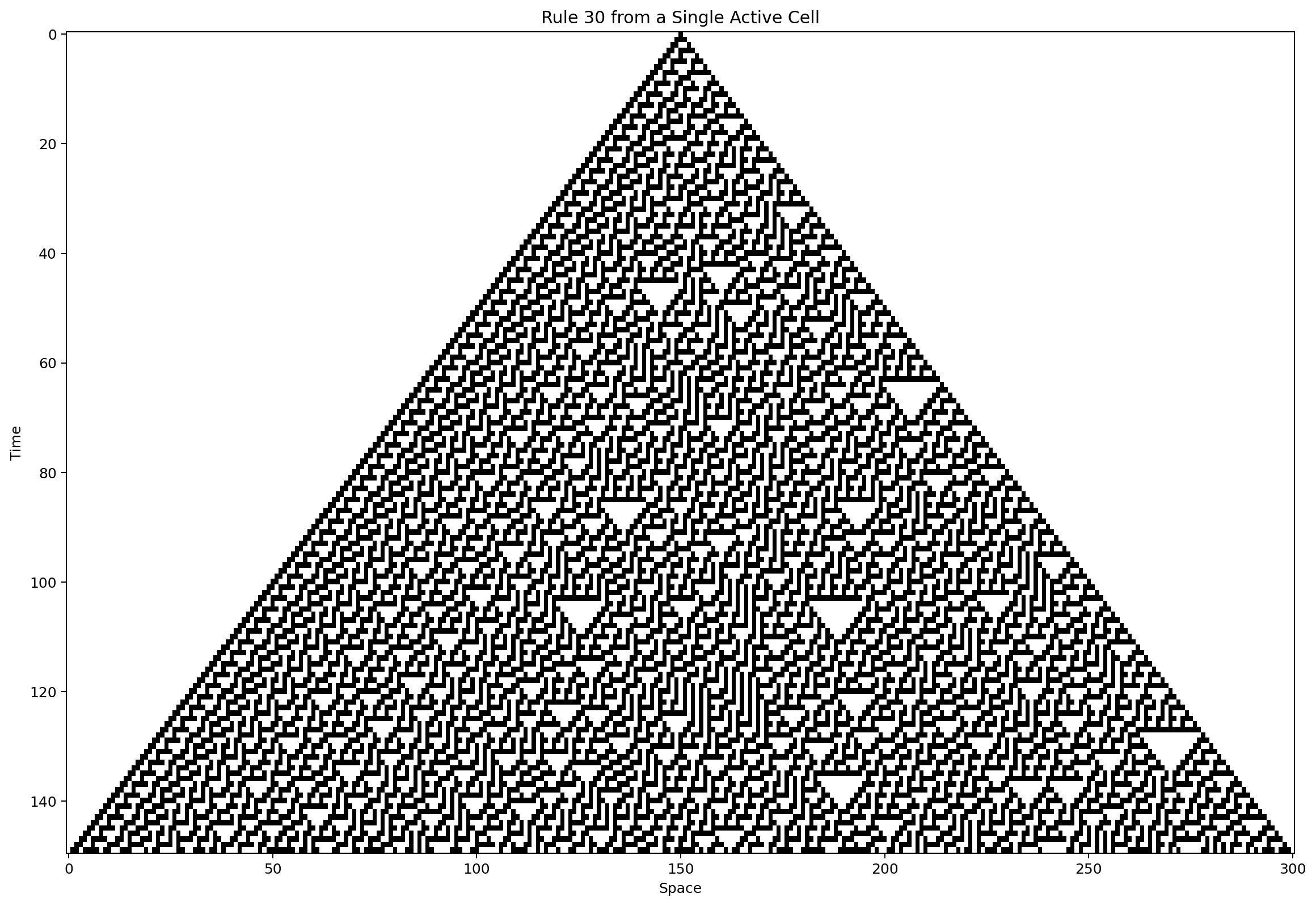
There is visible structure on the left.

There is irregularity on the right.

There are repeating fragments.

There are regions that look almost patterned and then break apart.

The entire thing is generated deterministically.

No random numbers are involved.

That is our first real surprise.

Nothing random happened

This matters.

Rule 30 does not roll dice.

At every location, the same local transformation is applied.

Its transition table is fixed:

111 → 0
110 → 0
101 → 0
100 → 1
011 → 1
010 → 1
001 → 1
000 → 0

That gives the binary output:

00011110

which is:

30

Every future state follows from:

rule
+
current state

There is no hidden source of noise.

If we begin from exactly the same initial condition, we get exactly the same history.

Every time.

So the irregularity in the image cannot be explained by saying:

randomness was injected.

It wasn’t.

Deterministic does not mean obvious

That distinction is easy to miss.

A deterministic system means:

given the current state, the next state is fixed.

It does not mean:

a human can easily predict the long-term result.

Those are completely different claims.

Consider this tiny operation:

next_state = step(state, rule=30)

Each individual update is trivial.

But after many updates, the result becomes difficult to anticipate by inspection.

We therefore need to separate:

local predictability

from:

global predictability

Locally, the rule is embarrassingly simple.

Globally, the trajectory is not.

Where is the complexity?

This question is more difficult than it sounds.

Is the complexity inside the rule?

Not obviously.

The rule has only eight output bits.

Is it inside the starting state?

We started with one active cell.

Is it inside the individual cells?

Each stores one bit.

So perhaps the interesting behavior lives somewhere else:

simple rule
+
simple state
+
repeated interaction
+
time

The structure appears in the unfolding.

This is one reason the word emergence is so tempting.

But we should be careful.

What does emergence mean here?

People often use emergence to mean:

something surprising happened.

That is too weak.

Surprise depends partly on the observer.

A system is not scientifically interesting merely because we failed to guess what it would do.

A stronger working idea is:

a macroscopic pattern or behavior arises from local interactions and is not explicitly represented in the individual components.

Under that definition, Rule 30 is at least a useful candidate.

The cells do not contain:

triangle
left edge
right-side irregularity
long-range structure

The local rule does not contain an explicit spacetime diagram.

Yet those structures appear when the system evolves.

That gives us something worth investigating.

Not proof of life.

Not proof of intelligence.

Not even proof of deep complexity.

Just evidence that:

simple local mechanics can generate nontrivial global organization.

That is enough for now.

Compare two rules

Let’s make the contrast explicit.

Take the same initial condition:

000000000010000000000

Run Rule 22.

Then run Rule 30.

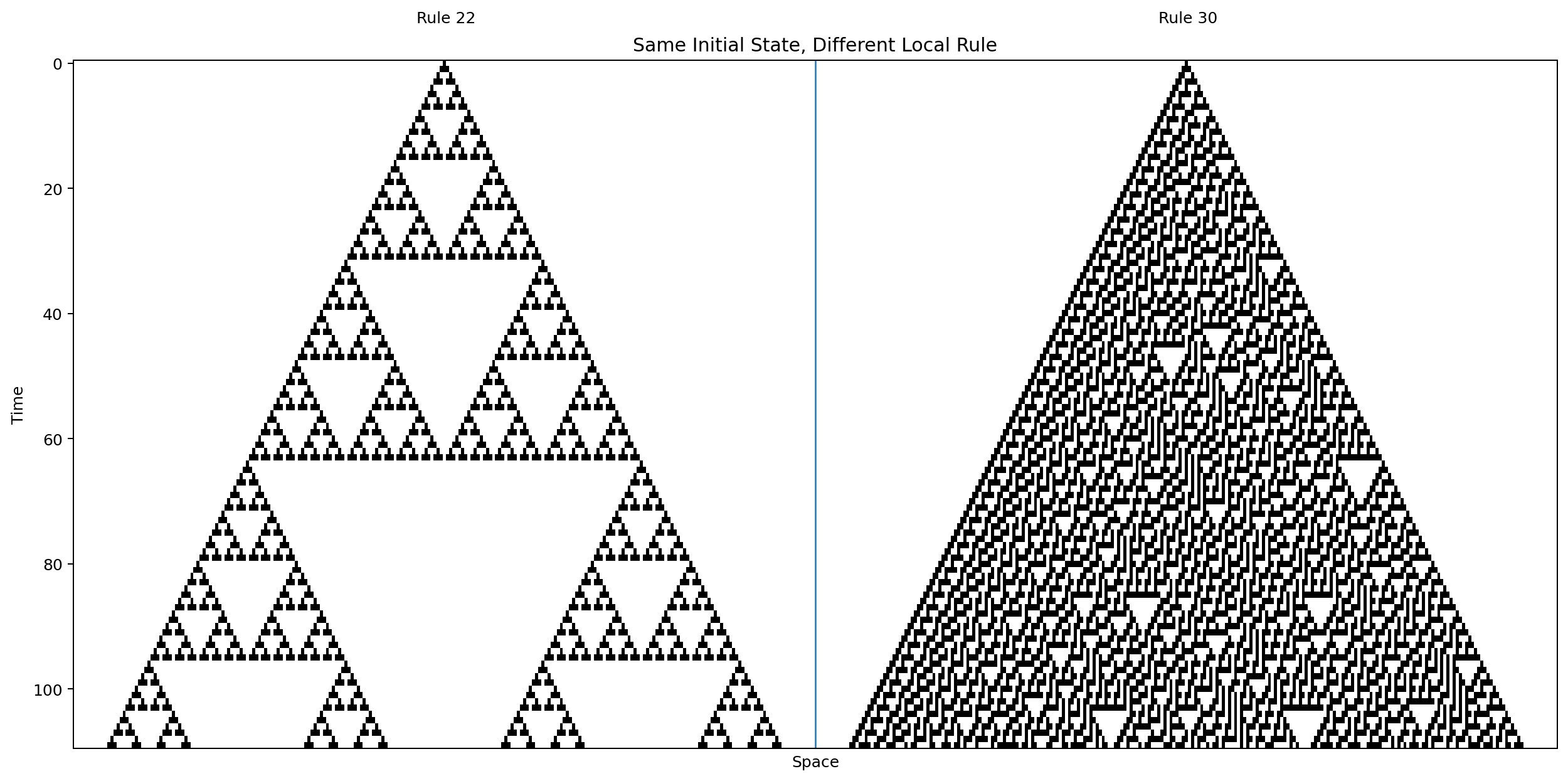
Everything except the rule remains fixed.

We are doing a controlled experiment.

Conceptually:

Experiment A
rule = 22

Experiment B
rule = 30

Same initial state.

Same boundary conditions.

Same world size.

Same number of generations.

The difference in behavior therefore comes from the rule.

That seems obvious, but this discipline will become increasingly important later when our systems contain many parameters.

Change one bit in the rule

Rule 30 is:

00011110

Suppose we flip a single output bit.

Now we might have:

00011111

or:

00010110

That gives us a neighboring rule in rule space.

The local mechanism has changed only slightly.

But the long-term behavior can change dramatically.

This suggests a useful experiment.

Rather than asking:

what does Rule 30 do?

ask:

how stable is Rule 30’s behavior under small changes to the rule itself?

That is a different question.

And it matters because eventually we will talk about mutation.

A mutation in a digital rule may be tiny in representation but enormous in consequence.

Change one bit in the world

We can perturb the initial condition too.

Start from:

000000000010000000000

Then compare it with:

000000000011000000000

One extra active cell.

Nothing else changes.

Now run both under Rule 30.

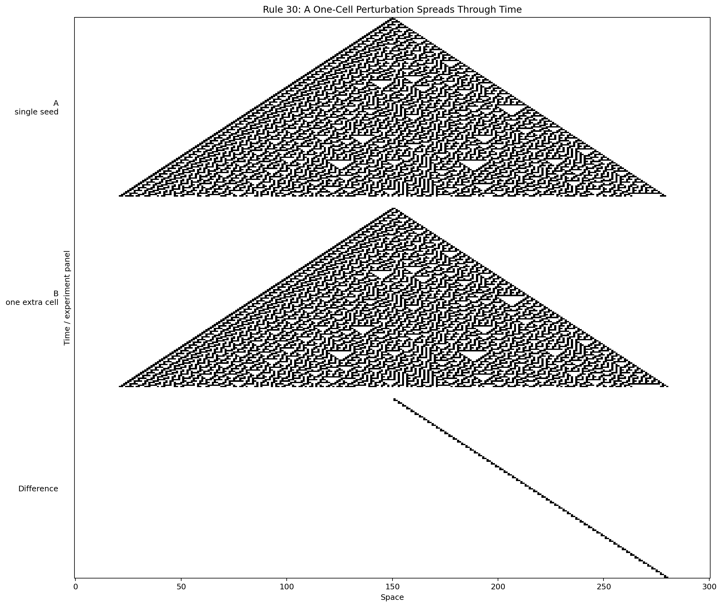
At first the difference is tiny.

Then it spreads.

The local disturbance affects nearby neighborhoods.

Those changed neighborhoods alter the next generation.

The difference propagates outward.

This gives us another candidate property:

sensitivity to initial conditions

Again, don’t overstate it.

We have not yet measured sensitivity.

We have only created an experiment that can expose it.

Later, we will quantify how quickly two nearby histories diverge.

A difference can move

Suppose we have two states:

A
00000100000

B
00000110000

Their difference is:

00000010000

One cell.

After one update, the two worlds may differ in several places.

Then more.

The difference itself becomes something we can track.

This is important.

We are no longer limited to studying visible patterns in one world.

We can study:

world A
world B
difference(A, B)

That difference field becomes an experimental instrument.

Later we can measure:

number of differing cells
fraction of differing cells
rate of divergence
spatial spread of perturbation

This is the beginning of turning pictures into evidence.

But isn’t this just chaos?

Maybe.

But we should not use that word casually either.

“Chaos” has technical meanings in dynamical systems.

A system looking irregular is not automatically chaotic.

Likewise:

irregular
random
chaotic
complex
emergent

are not synonyms.

A good rule for this book is:

If a word sounds impressive, define the measurement before trusting the word.

For now, Rule 30 is:

• deterministic,
• generated by a local rule,
• visually irregular in part of its spacetime diagram,
• sensitive enough to motivate perturbation experiments.

That’s plenty.

The danger of the screenshot

This deserves its own warning.

Suppose I show you this:

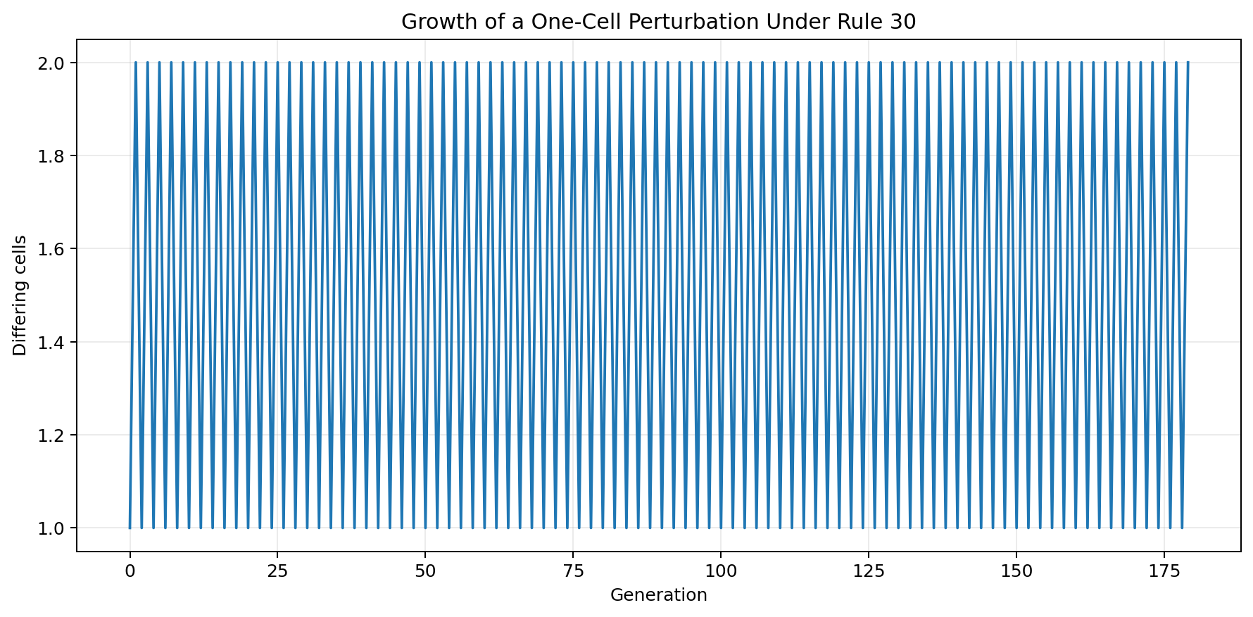
and say:

Look how complex it is.

That proves almost nothing.

I chose the rule.

I chose the initial condition.

I chose the crop.

I chose the number of generations.

I chose the rendering.

I could easily show you only the most impressive region.

This is the same problem we will encounter later with artificial-life organisms.

A spectacular example is useful for discovering a phenomenon.

It is weak evidence for how general that phenomenon is.

So eventually we will need to ask:

How often does this behavior occur?

Across which rules?

Across which starting states?

How sensitive is it?

How persistent is it?

Can we measure it without hand-picking examples?

That is where search and measurement enter.

Rule 30 has another strange property

Look at the central column of the spacetime diagram.

If we record one cell through time, we obtain a binary sequence:

0
1
1
0
1
0
...

A tiny deterministic cellular automaton can therefore be used as a generator of complicated-looking bit sequences.

This is historically interesting, but more important for us conceptually.

The spatial system can be observed in another way.

Instead of looking at:

the whole world at one time

we can look at:

one location across many times

The same system supports multiple observables.

This will matter enormously later.

What we conclude about a system depends partly on what we measure.

One system, many descriptions

Rule 30 can be described as:

an eight-bit lookup table

or:

a one-dimensional cellular automaton

or:

a spacetime pattern

or:

a generator of temporal bit sequences

or:

a dynamical system moving through a large state space

None of these descriptions is necessarily wrong.

They emphasize different levels.

This is a recurring theme in Digital Life.

A future system might simultaneously be describable as:

a field update equation

a self-maintaining pattern

a learned dynamical system

an evolutionary lineage

The challenge is knowing which claims are supported at which level.

Let’s inspect the rule itself

There is something almost insulting about how small Rule 30 is.

We can print its entire behavior in eight lines.

rule = {
    (1, 1, 1): 0,
    (1, 1, 0): 0,
    (1, 0, 1): 0,
    (1, 0, 0): 1,
    (0, 1, 1): 1,
    (0, 1, 0): 1,
    (0, 0, 1): 1,
    (0, 0, 0): 0,
}

That is the whole law.

There is no hidden complexity waiting below it.

The complexity appears only after we allow those local interactions to repeat.

This gives us the first major result of the book:

A globally nontrivial trajectory does not require a globally complicated controller.

That result is modest.

But it is foundational.

We still don’t have a thing

Rule 30 produces structure.

But does it produce an entity?

Something with an identity?

Something we can point at and say:

that thing persisted.

Not obviously.

The pattern expands.

Regions change.

Information appears to propagate.

But identifying a stable localized object is harder.

So we need another system.

One where patterns do not merely spread across a spacetime diagram.

One where a structure can appear here:

.##.
##..
....

and later appear somewhere else while remaining recognizably the same organization.

That brings us to Conway’s Game of Life.

And to a much stranger question:

When does a pattern become a thing?

Next: When Does a Pattern Become a Thing?