Digital Life 05: Kill It

We have been too kind to our systems.

So far we have:

• initialized them carefully,
• given them clean environments,
• watched them evolve,
• selected examples that behave interestingly,
• and mostly left them alone.

That is a dangerous way to study anything that looks life-like.

A structure that persists when nothing interferes with it may be interesting.

But biological systems do something harder.

They persist in a world that keeps interfering with them.

So let’s interfere.

Start with the glider

Our glider:

.#.
..#
###

moves through Conway’s Game of Life as a dynamically persistent localized pattern.

After four generations it reproduces its orientation one cell diagonally away.

That gave us a useful definition of persistence.

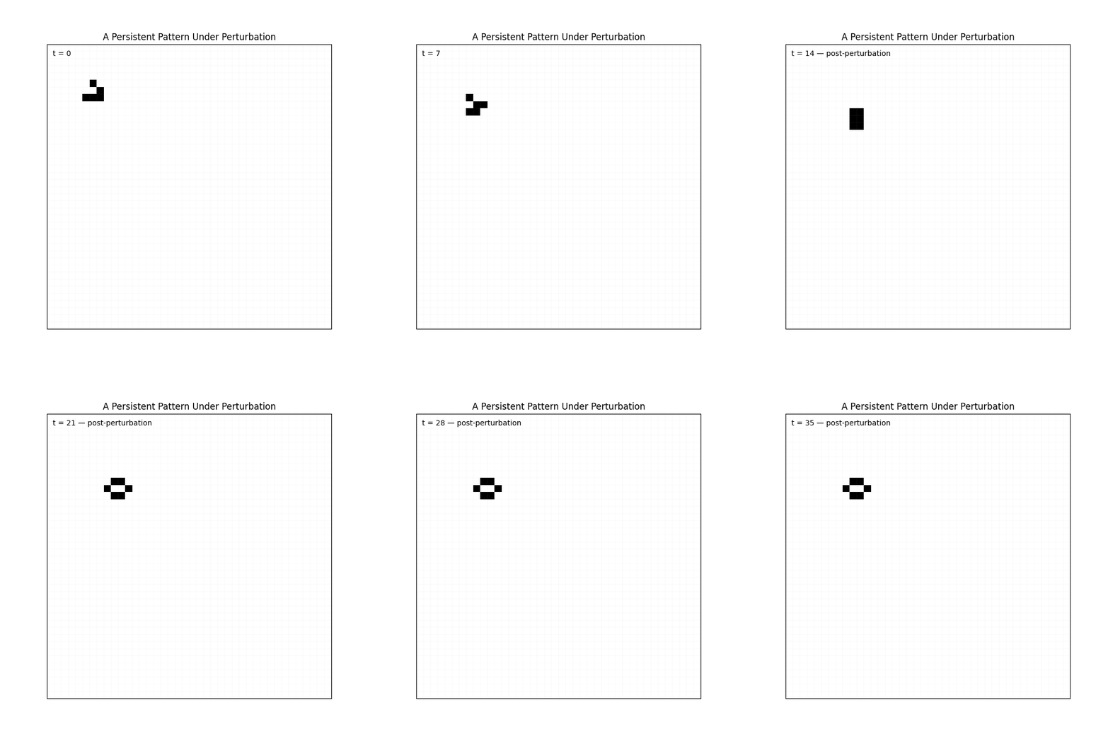
Now remove one cell.

For example:

.#.
...
###

One bit changed.

Run the same rule.

Same world.

Same boundary conditions.

Same update semantics.

Only the initial structure has changed.

What happens?

Perhaps the pattern disappears.

Perhaps it becomes another Life pattern.

Perhaps some debris persists.

What does not happen is equally important:

the original glider does not necessarily reconstruct itself.

That immediately tells us something.

Persistence under normal evolution does not imply recovery after damage.

Three different claims

We need to stop using one vague word for several different properties.

Consider these three systems.

System A

It remains unchanged forever if nothing disturbs it.

That is:

persistence

System B

Small disturbances do not destroy its overall behavior.

That is:

robustness

System C

A disturbance changes its structure, but the system subsequently reconstructs something sufficiently close to its earlier organization.

That is:

regeneration

These are not synonyms.

Write them separately:

persistence
≠
robustness
≠
regeneration

A system can have one without the others.

A block persists

Take the Game of Life block:

##
##

Under ordinary Life evolution:

t = 0

##
##

t = 1

##
##

t = 2

##
##

It is perfectly persistent.

Now delete one cell:

#.
##

Run one generation.

The remaining structure disappears.

So the block has excellent undisturbed persistence and terrible tolerance to this particular perturbation.

The experiment exposes a property the clean simulation hid.

A perturbation is part of the experiment

This sounds obvious, but it changes how we think about these systems.

Our experiment is no longer merely:

initial state
    ↓
evolution
    ↓
final state

It becomes:

initial state
    ↓
stable behavior
    ↓
controlled perturbation
    ↓
response
    ↓
measurement

The perturbation is not noise around the experiment.

It is the experiment.

Damage must be defined

“Damage the organism” sounds intuitive.

It is also scientifically useless until we specify what damage means.

For a binary cellular automaton, we might define damage as:

flip one active cell to inactive

or:

flip N randomly chosen cells

or:

erase every cell inside a square region

or:

replace a fraction of the pattern with random states

Each is a different intervention.

So a proper damage protocol might be:

pattern: glider
damage time: t = 20
damage type: delete active cells
damage amount: 1 cell
damage location: leading edge
trials: all possible active-cell deletions

Now someone else can reproduce what we did.

One successful recovery proves very little

Imagine a pattern with ten active cells.

We delete one particular cell.

The pattern recovers.

Wonderful.

But what if deleting any of the other nine cells destroys it?

Then:

“the system regenerates after damage”

would be misleading.

A stronger experiment tries many perturbations.

For example:

for cell in active_cells:
    damaged = state.copy()
    damaged[cell] = 0

    result = run(damaged)

    measure_recovery(result)

Now we can ask:

How many perturbations were survivable?

Which locations were critical?

How much structure was lost?

How long did recovery take?

The system begins to acquire a damage profile.

Survival is not recovery

Suppose we damage a structure and it continues to exist.

That does not mean it regenerated.

Imagine:

before

.###.
##.##
.###.

after damage

.#...
##...
.....

Twenty generations later:

##...
##...
.....

Something survived.

But the original organization did not return.

So:

nonzero activity

is not enough.

Nor is:

localized activity

enough.

To claim recovery, we need some relationship between:

structure before damage

and:

structure after recovery

What counts as “the same”?

Game of Life gives us a clean version of this problem.

For exact discrete patterns, we might compare states directly.

np.array_equal(before, after)

But that fails for moving patterns.

A recovered glider might be shifted.

So perhaps we compare:

same structure
up to translation

For an oscillator:

same structure
up to phase

Later, in continuous artificial-life systems, exact equality will become unrealistic.

Then we may need:

shape similarity
mass similarity
spatial overlap
feature similarity
behavioral similarity

Notice what is happening.

The moment we ask whether something regenerated, we are forced to define what we mean by its identity.

The philosophical question from the previous chapter becomes an engineering requirement.

Define a recovery score

Suppose we have a target pattern:

T

and a recovered pattern:

R

A simple binary similarity score might measure the fraction of cells that match after alignment.

For example:

def similarity(a, b):
    return np.mean(a == b)

But this has a problem.

If almost every cell in the world is zero, two completely different tiny patterns could still receive a very high score.

So the metric must focus on the relevant region or structure.

Perhaps we measure:

intersection
union

of active cells.

One possible score is intersection-over-union:

IoU =
active in both
-------------
active in either

Now identical active regions score:

1.0

and disjoint patterns score:

0.0

Better.

Still not universally correct.

But at least explicit.

Metrics create claims

Suppose we define:

recovered =
IoU >= 0.90
within 50 generations

Now our claim can be:

Under this damage protocol, the pattern returned to at least 0.90 IoU with its pre-damage morphology within 50 updates.

That is ugly compared with:

It healed itself.

Good.

Ugly claims are often safer.

We can always summarize later.

But the experiment should preserve the operational statement.

Robustness can mean something weaker

A system may fail to reconstruct its exact morphology yet preserve its function.

Imagine a future digital organism whose task is:

move toward a resource source

Damage changes its shape.

But it still moves toward the resource.

Morphological similarity could be low while functional performance remains high.

That suggests two different recovery questions:

Did the structure recover?

and:

Did the capability recover?

Those are not necessarily the same.

Later we will need both.

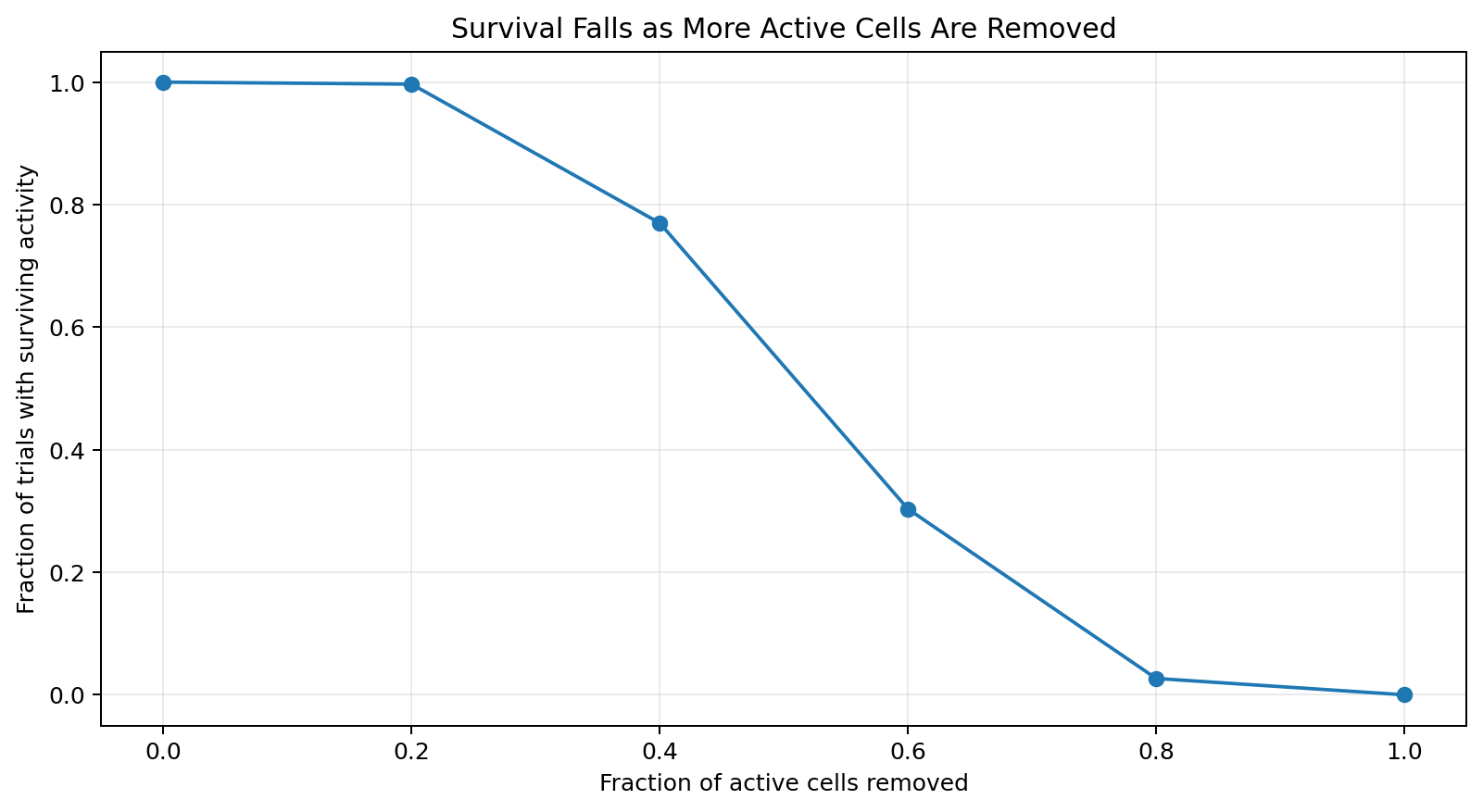
A damage curve

Instead of one perturbation, increase the severity.

For example:

0% removed
5% removed
10% removed
20% removed
40% removed
60% removed

For each level:

1. damage the system,
2. run it,
3. measure survival,
4. measure structural recovery,
5. repeat across locations or random seeds.

Then plot:

damage severity
        ↓
recovery score

Now robustness stops being:

this thing seems tough.

It becomes a relationship.

Some systems might tolerate tiny perturbations and collapse suddenly.

Others may degrade gradually.

Still others may recover across a broad range.

Those response curves tell us much more than a clean animation.

Damage location matters

Imagine a large pattern.

Removing 10% of its cells from one region may have almost no effect.

Removing the same number from another region may destroy it.

So damage severity alone is insufficient.

We also need:

where?

This allows us to ask whether a system has:

fragile regions
redundant regions
critical structures
distributed organization

Later, when we study learned cellular automata, this becomes extremely interesting.

Does information live everywhere?

Or are there regions without which recovery becomes impossible?

Repeated damage is harder

Suppose a system recovers once.

Damage it again.

Then again.

A system could possess enough redundancy to survive one intervention but progressively lose its ability to recover.

So another protocol is:

damage
↓
recover
↓
damage
↓
recover
↓
damage
↓
recover

Measure whether performance declines.

Now we’re testing sustained robustness rather than one lucky recovery.

The environment can be the perturbation

Damage does not have to mean deleting cells.

A perturbation could be:

change temperature parameter
change resource availability
introduce another pattern
alter boundary conditions
inject noise
change update frequency
shift the objective

The deeper idea is:

A property becomes more convincing when it survives variation in conditions.

This principle will recur everywhere.

If a learned rule only works under the exact condition it was trained on, its apparent intelligence may be brittle.

If an evolved organism only survives in one hand-selected world, its adaptation may be narrow.

If inherited knowledge only helps on the same task that produced it, we may merely be copying answers.

Perturbation exposes the boundary of the claim.

The glider fails our stronger test

Return to our glider.

It is beautiful.

It is localized.

It moves.

Its organization persists through changing cells.

But if we alter the wrong cell, its characteristic trajectory is destroyed.

That does not make the glider uninteresting.

It makes the description more accurate.

We can say:

The glider demonstrates translating dynamic persistence under undisturbed Game of Life dynamics.

We should not say:

The glider demonstrates self-maintaining robust organization.

Those are different achievements.

And now we know how to distinguish them.

Could a local system actually regenerate?

Now the obvious question becomes interesting.

Can we construct a system where:

target structure
      ↓
damage
      ↓
local interactions
      ↓
target structure returns

without a central controller holding a blueprint and simply repainting the missing pieces?

Yes.

Later in the book we will build learned neural cellular automata that can do something much closer to this.

They will begin from local rules.

We will damage the resulting morphology.

And the learned dynamics can sometimes restore it.

But when we get there, we will not simply show a GIF and declare:

healing!

We now know the questions to ask.

How much damage?

Which regions?

How many trials?

How complete was recovery?

How quickly?

Compared with what baseline?

Does it generalize to damage patterns not used during training?

The flashy experiment comes later.

The measurement rules come first.

This is why we damage things

There is a general method hiding here.

Whenever a system appears to possess a capability:

persistence
memory
adaptation
regeneration
generalization
inheritance

don’t merely observe the capability in the condition that produced it.

Attack the condition.

For memory:

remove or corrupt the stored state.

For inheritance:

compare successors with and without it.

For adaptation:

change the environment.

For regeneration:

damage the structure.

For robustness:

increase the perturbation.

For evolution:

evaluate on unseen environments.

The intervention tells us whether the mechanism is doing real work.

Our experimental vocabulary is growing

We started this book with:

state
+
local interaction
+
time

Now we have added:

intervention

So our laboratory increasingly looks like:

system
    ↓
observation
    ↓
controlled perturbation
    ↓
response
    ↓
measurement
    ↓
bounded claim

That is much closer to the method we will need for digital life.

But damage raises another question

Suppose a system is damaged beyond recovery.

Suppose it disappears.

Fine.

But what if, before disappearing, it produces another pattern?

Or another pattern emerges nearby that resembles it?

Or a structure produces copies of itself before any damage occurs?

Persistence concerns one continuing organization.

Reproduction changes the problem.

Now the system does not need one instance to last forever.

Information can persist through successors.

That is much closer to what biology actually does.

And it creates a whole new set of traps.

A pattern that copies itself is not automatically evolving.

A duplicate is not automatically offspring.

A mutation is not automatically adaptation.

And reproduction without useful inheritance may accomplish very little.

So now that we know how to kill a pattern, let’s ask whether it can avoid the problem another way.

By making another one.

Next: Can It Make Another One?