Encode All 256 Elementary Rules
Cellular Automata From First Principles 02: Encode All 256 Elementary Rules
An elementary cellular automaton has only three inputs per cell:
left centre right
Each input is one bit.
That means there are only eight possible neighborhoods:
111 110 101 100 011 010 001 000
For each neighborhood the rule chooses either 0 or 1.
Eight binary choices means:
2^8 = 256
possible rules.
The elegant part is that we can store one complete rule table in one byte.
Rule numbers are lookup tables
Take Rule 30.
Thirty in eight-bit binary is:
00011110
Read those bits against the neighborhoods in descending order:
| Neighborhood | Output |
|---|---|
| 111 | 0 |
| 110 | 0 |
| 101 | 0 |
| 100 | 1 |
| 011 | 1 |
| 010 | 1 |
| 001 | 1 |
| 000 | 0 |
So the rule number is not a mysterious label.
It is the transition table encoded as an integer.
    flowchart LR
    A[Rule number] --> B[8-bit binary table]
    B --> C[Neighborhood outputs]
    C --> D[Shared local transition]
Turn a neighborhood into an index
A three-bit neighborhood already has a natural integer value:
000 -> 0
001 -> 1
010 -> 2
011 -> 3
100 -> 4
101 -> 5
110 -> 6
111 -> 7
We can compute that without strings:
def neighborhood_index(left, centre, right):
    return (left << 2) | (centre << 1) | right
Then extract the corresponding bit from the rule number:
def elementary_rule(rule_number, left, centre, right):
    index = neighborhood_index(left, centre, right)
    return (rule_number >> index) & 1
That one function can execute any elementary rule from 0 to 255.
There is a useful consistency check here. For Rule 30, neighborhood 100 has index 4, so:
(30 >> 4) & 1 = 1
which matches the table above.
A complete simulator
import numpy as np


def step(state, rule_number):
    next_state = np.zeros_like(state)

    for i in range(len(state)):
        left = state[(i - 1) % len(state)]
        centre = state[i]
        right = state[(i + 1) % len(state)]
        next_state[i] = elementary_rule(
            rule_number, left, centre, right
        )

    return next_state


def run(rule_number, width=101, generations=100):
    state = np.zeros(width, dtype=np.uint8)
    state[width // 2] = 1

    history = [state.copy()]

    for _ in range(generations - 1):
        state = step(state, rule_number)
        history.append(state.copy())

    return np.array(history)
Now exploring a different automaton is just:
history = run(30)
or:
history = run(110)
or:
history = run(184)
The engine stays fixed.
Only the local law changes.
Generate every rule
import matplotlib.pyplot as plt

fig, axes = plt.subplots(16, 16, figsize=(16, 16))

for rule_number, ax in enumerate(axes.flat):
    history = run(rule_number, width=63, generations=40)
    ax.imshow(history, cmap="binary", interpolation="nearest")
    ax.set_title(str(rule_number), fontsize=6)
    ax.axis("off")

plt.tight_layout()
plt.show()
The book’s reproducible figure script generates the same experiment as a canonical asset:
python scripts/figures/cellular-automata/part01_foundations.py 02
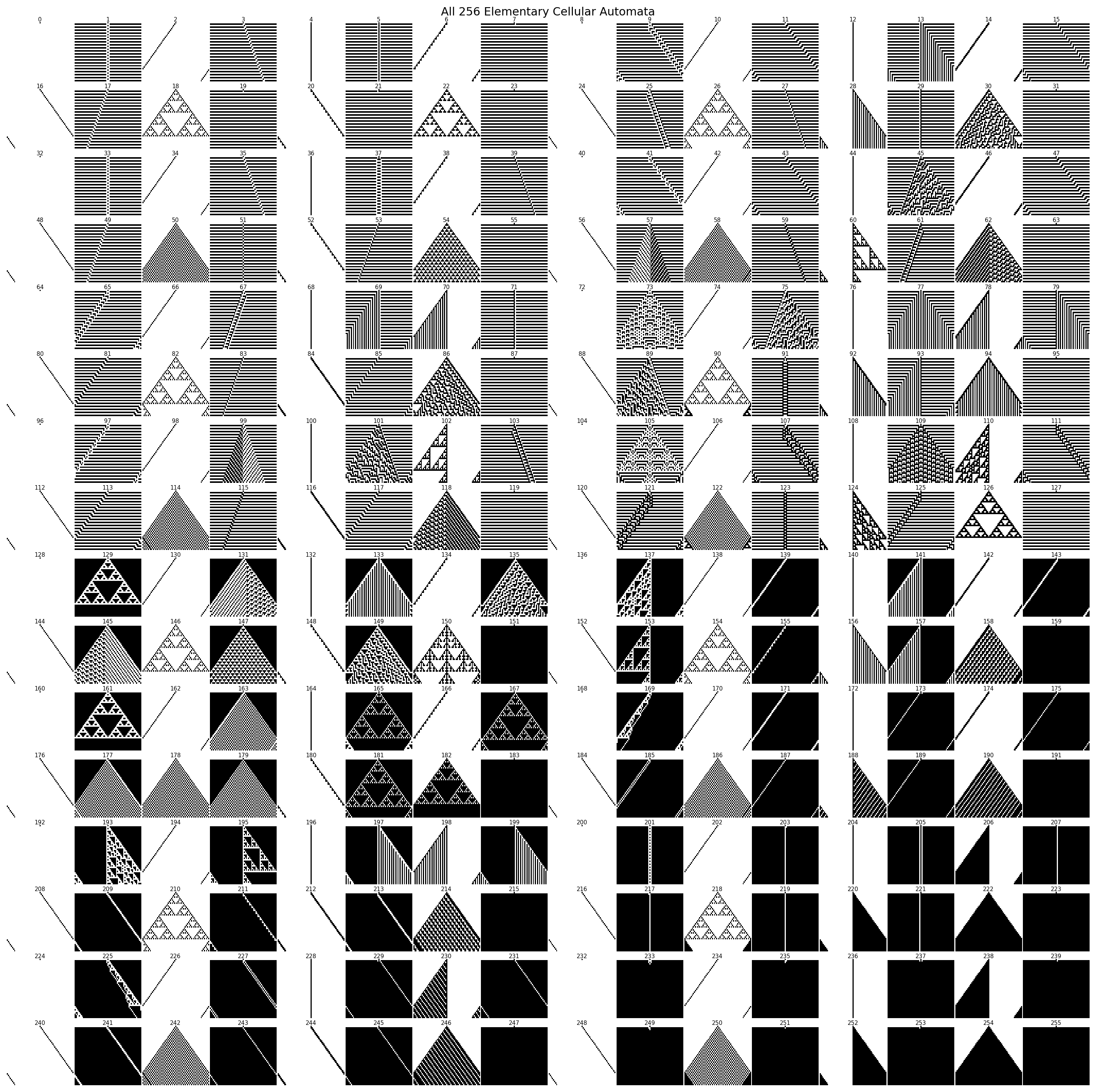
This is one of the best experiments in the subject.
The rules have exactly the same:
- grid,
- state space,
- neighborhood,
- initial condition,
- execution engine.
Only eight output bits differ.
Yet the resulting systems look radically different.
That is emergence in a form we can inspect directly.
Compare rules by measurements, not just pictures
A visual catalog is useful, but we can also measure the histories.
Density
def density(history):
    return history.mean(axis=1)
This tells us what fraction of cells are active at each generation.
Change rate
def change_rate(history):
    return np.mean(history[1:] != history[:-1], axis=1)
This measures how much each generation differs from the previous one.
Spatial entropy
For a binary row with active-cell probability p:
import numpy as np


def binary_entropy(row):
    p = row.mean()
    if p in (0.0, 1.0):
        return 0.0
    return -(p * np.log2(p) + (1 - p) * np.log2(1 - p))
This quantity measures the balance between zeros and ones in one row. It does not by itself measure spatial organization: two rows with the same density have the same binary entropy even if one contains long blocks and the other alternates rapidly.
That limitation is useful. It teaches us to ask what a metric actually observes rather than giving a number more meaning than it has.
These are crude measurements, but they change the question from:
Which rule looks complicated?
to:
Which observable properties distinguish one dynamical regime from another?
That is a much stronger habit.
Initial conditions matter too
A single central cell is convenient, but it is not the whole story.
Try a random state:
rng = np.random.default_rng(42)
state = rng.integers(0, 2, size=101, dtype=np.uint8)
Or a repeating pattern:
state = np.resize(np.array([1, 0, 0], dtype=np.uint8), 101)
A cellular automaton is a dynamical system.
The behavior belongs to the combination:
rule + initial state + boundary conditions + update scheme
not to the rule number alone.
The important abstraction
We can now separate the system into three pieces:
encoding
  rule number -> transition table

runtime
  neighborhood -> update -> next generation

experiment
  initial state + duration + measurements
That is already enough to build a serious exploration tool.
In the next chapter we will focus on one of the most famous rules in the catalog: Rule 30.
Its local rule is tiny.
Its global pattern looks anything but tiny.
