Cellular Automata From First Principles 05: Conway’s Game of Life

Conway’s Game of Life is one of the cleanest examples of complex two-dimensional behavior emerging from a tiny local rule.

The world is a grid of dead and live cells.

Each cell sees its eight surrounding neighbors.

Then four ideas decide the next generation:

underpopulation
survival
overpopulation
birth

The standard rule is usually written B3/S23:

• a dead cell is born with exactly 3 live neighbors,
• a live cell survives with 2 or 3 live neighbors.

Everything else becomes or remains dead.

Represent the grid

import numpy as np

grid = np.zeros((40, 60), dtype=np.uint8)

Seed a simple three-cell line:

grid[20, 29:32] = 1

That pattern is the blinker.

Count neighbors with array shifts

We can count all eight neighbors using np.roll:

def neighbor_count(grid):
    total = np.zeros_like(grid, dtype=np.uint8)

    for dy in (-1, 0, 1):
        for dx in (-1, 0, 1):
            if dx == 0 and dy == 0:
                continue
            total += np.roll(np.roll(grid, dy, axis=0), dx, axis=1)

    return total

This gives periodic boundaries: the top connects to the bottom and the left edge connects to the right.

Now implement B3/S23:

def life_step(grid):
    n = neighbor_count(grid)

    born = (grid == 0) & (n == 3)
    survive = (grid == 1) & ((n == 2) | (n == 3))

    return (born | survive).astype(np.uint8)

That is the complete Game of Life rule.

The same synchronous-update discipline from our one-dimensional automata still applies: every birth and death is calculated from the same current generation.

Watch an oscillator

for generation in range(4):
    print(f"generation {generation}")
    print(grid[18:23, 27:34])
    grid = life_step(grid)

The blinker alternates between horizontal and vertical states.

So we have discovered our first attractor cycle:

state A -> state B -> state A -> ...

Seed a glider

glider = np.array([
    [0, 1, 0],
    [0, 0, 1],
    [1, 1, 1],
], dtype=np.uint8)

grid = np.zeros((60, 80), dtype=np.uint8)
grid[5:8, 5:8] = glider

Repeated Life updates cause the pattern to reproduce its shape at an offset.

The canonical static figure shows four phases of that motion:

python scripts/figures/cellular-automata/part01_foundations.py 05

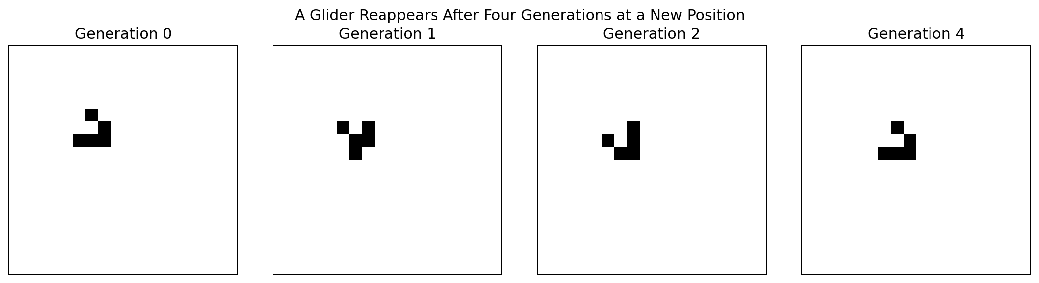
After four generations the glider has the same orientation but is shifted one cell diagonally.

That means a local configuration has become a moving object.

No code says:

glider.move_diagonally()

Movement is an emergent property of repeated births and deaths.

Animate the simulation

import matplotlib.pyplot as plt
from matplotlib.animation import FuncAnimation

fig, ax = plt.subplots()
image = ax.imshow(grid, cmap="binary", interpolation="nearest")
ax.axis("off")


def update(_):
    global grid
    grid = life_step(grid)
    image.set_data(grid)
    return (image,)

animation = FuncAnimation(fig, update, interval=80, blit=True)
plt.show()

The animation is useful, but keep the transition function separate from rendering.

That gives us:

model -> state transition
view  -> visualization

and prevents display code from defining the simulation.

Classify patterns by behavior

Life produces several broad kinds of structure.

Still lifes

Patterns that stop changing.

Examples include blocks and beehives.

Oscillators

Patterns that repeat after a fixed period.

The blinker has period two.

Spaceships

Patterns that repeat after a fixed number of generations but at a translated position.

The glider is the canonical example.

Methuselahs

Small initial patterns that evolve for a surprisingly long time before settling into simpler debris.

These categories are useful because they describe dynamics, not merely shape.

Measure population through time

def simulate_life(grid, steps):
    history = []
    state = grid.copy()

    for _ in range(steps):
        history.append(state.copy())
        state = life_step(state)

    return history

history = simulate_life(grid, 200)
population = [state.sum() for state in history]

plt.plot(population)
plt.xlabel("generation")
plt.ylabel("live cells")
plt.show()

Population alone cannot tell us what structures exist, but it is one useful observable.

We can add:

• bounding-box size,
• number of connected components,
• period detection,
• translation detection,
• entropy,
• collision outcomes.

This is how we move from watching Life to analyzing Life.

The deeper programming lesson

A glider looks like an object.

But there is no glider object in the implementation.

There are only cells and a local update rule.

That distinction is important:

implementation ontology:
    cells + rules

observer ontology:
    gliders + blinkers + spaceships

Higher-level entities can be real and useful even when they are not primitive objects in the code.

That is one of the most important ideas in emergent systems.

In the next chapter we will exploit that idea directly: we will build a small library of Life patterns, detect oscillation and movement, and treat recurring structures as data.