Activity, Density and Change
Cellular Automata From First Principles 18: Activity, Density and Change
A cellular automaton can look busy while doing very little that persists.
It can also look visually quiet while preserving a small moving structure for hundreds of generations.
So we need to separate several properties that are easy to confuse:
occupancy
temporal change
spatial variation
persistence
This chapter turns those ideas into explicit measurements.
Together they form our first useful behavioral fingerprint.
Density measures occupancy
For a binary state:
def density(state):
    return float(state.mean())
Density answers:
What fraction of the world is active?
Compare:
11110000
10101010
Both have:
density = 0.5
But their spatial organization is completely different.
So density tells us how much state is active.
It does not tell us how that state is arranged or whether it is changing.
Activity measures temporal change
Define activity as the fraction of cells that changed since the previous generation:
def activity(previous, current):
    return float(
        np.mean(previous != current)
    )
Now some obvious cases become measurable:
activity = 0
    no cell changed

activity ≈ 1
    almost every cell changed

0 < activity < 1
    only part of the world changed
Across a complete trajectory:
def activity_curve(history):
    return np.mean(
        history[1:] != history[:-1],
        axis=1,
    )
This gives us:
generation -> fraction of cells changed
The curve matters more than one final value.
A rule may be highly active early and completely frozen later.
Transient activity is not persistent activity
Consider two runs.
Run A
generations 0-30:
    high activity

generations 31-500:
    activity = 0
Run B
generations 0-500:
    moderate activity
Their mean activity could be surprisingly similar over a short experiment.
But dynamically they are very different.
So measure late-run activity separately:
import numpy as np


def tail_activity(
    history,
    tail=50,
):
    curve = activity_curve(history)

    if len(curve) == 0:
        return 0.0

    return float(
        np.mean(curve[-tail:])
    )
This gives us a simple distinction:
early activity
    -> transient dynamics

tail activity
    -> sustained dynamics
That distinction will become increasingly important when we search rule spaces.
Count how often each cell changes
Global activity tells us how much of the world changes.
It does not tell us where the change occurs.
Count transitions at each position:
def cell_change_counts(history):
    return np.sum(
        history[1:] != history[:-1],
        axis=0,
    )
Now each cell gets a value:
0
    never changed

5
    changed five times

100
    changed repeatedly
For an elementary automaton started from one active cell, these counts often reveal the expanding causal region directly.
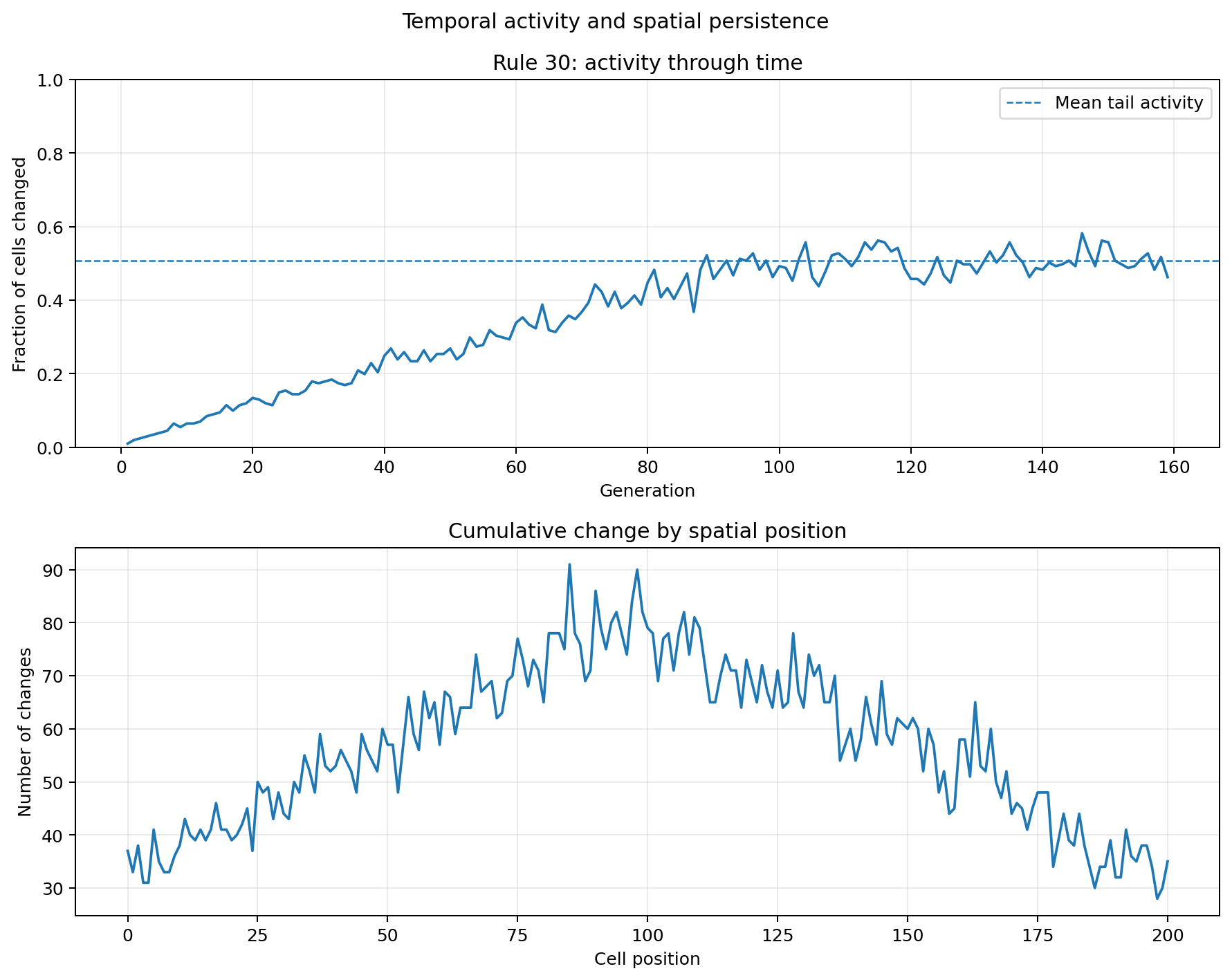
The ordinary spacetime diagram shows the state.
The change-count view shows where dynamics actually occurred.
Detect extinction and saturation explicitly
Binary automata have two particularly simple global states:
all 0
all 1
Detect them directly:
def terminal_state(state):
    if np.all(state == 0):
        return "empty"

    if np.all(state == 1):
        return "full"

    return "mixed"
This gives search pipelines a cheap first filter.
Rules that immediately become completely empty or full may still be worth understanding, but we do not need expensive measurements to discover that they reached a trivial homogeneous state.
Spatial variation measures local disagreement
Density ignores arrangement.
So measure neighboring differences:
def spatial_variation(state):
    right = np.roll(state, -1)

    return float(
        np.mean(state != right)
    )
Compare:
0000000011111111
with:
0101010101010101
Both can have density 0.5.
But the second changes at almost every neighboring boundary.
Spatial variation distinguishes that organization.
Extend spatial variation to two dimensions
For a 2D grid:
def spatial_variation_2d(grid):
    horizontal = np.mean(
        grid
        != np.roll(
            grid,
            -1,
            axis=1,
        )
    )

    vertical = np.mean(
        grid
        != np.roll(
            grid,
            -1,
            axis=0,
        )
    )

    return float(
        (horizontal + vertical) / 2
    )
Again, the metric is simple.
It is not a universal measure of structure.
It answers one specific question:
How often do neighboring cells disagree?
That specificity is a strength.
Build a behavioral fingerprint
We now have several different observables.
Combine them:
def fingerprint(history):
    activities = activity_curve(history)

    return {
        "mean_density": float(
            np.mean(history)
        ),
        "final_density": float(
            density(history[-1])
        ),
        "mean_activity": float(
            np.mean(activities)
        ) if len(activities) else 0.0,
        "tail_activity": tail_activity(
            history
        ),
        "spatial_variation": (
            spatial_variation(
                history[-1]
            )
        ),
        "terminal": terminal_state(
            history[-1]
        ),
    }
Now a rule does not receive one vague label such as:
complex
It receives a vector of observable properties.
Conceptually:
rule
  ↓
trajectory
  ↓
[
    density,
    activity,
    persistence,
    spatial variation,
    terminal behavior
]
That vector can later become input to:
clustering
classification
search
ranking
visualization
Compare fingerprints, not screenshots
Suppose two rules both look irregular.
Their fingerprints might reveal:
Rule A
mean activity:       high
tail activity:       near zero
spatial variation:   high

Rule B
mean activity:       moderate
tail activity:       moderate
spatial variation:   moderate
Now we know something important.
Rule A creates a violent transient and then settles.
Rule B maintains ongoing dynamics.
A screenshot taken at generation 20 might make them look similar.
A trajectory-level measurement separates them.
Evaluate several initial conditions
A rule is not fully characterized by one initial state.
Run the same rule from several random initial conditions:
def evaluate_rule(
    rule_number,
    seeds,
    width=201,
    generations=200,
):
    records = []

    for seed in seeds:
        history = run_rule(
            rule_number,
            width=width,
            generations=generations,
            seed=seed,
            initial="random",
        )

        records.append(
            fingerprint(history)
        )

    return records
Now calculate:
mean metric value
variance across runs
minimum
maximum
A rule whose measurements vary dramatically across initial conditions behaves differently from one whose fingerprint is extremely stable.
Later we will study that sensitivity directly.
Preserve the experimental context
A fingerprint without context can be misleading.
Record:
rule
initial-condition type
seed
width
generations
boundary condition
measurement version
For example:
record = {
    "rule": 30,
    "initial": "random",
    "seed": 42,
    "width": 201,
    "generations": 200,
    "boundary": "periodic",
    "features": fingerprint(history),
}
Now our feature vector remains tied to the experiment that produced it.
Metrics are features, not truth
A high-activity rule is not automatically interesting.
A low-activity rule is not automatically simple.
A checkerboard has high spatial variation while remaining highly regular.
A transient explosion can produce high mean activity without persistent dynamics.
So the correct pipeline is:
observation
    ↓
measurement
    ↓
comparison
    ↓
hypothesis
    ↓
another experiment
not:
single metric
    ↓
final interpretation
One idea to keep
Density tells us how much state is active.
Activity tells us how much state is changing.
Spatial variation tells us how locally fragmented the state is.
Persistence tells us whether the dynamics survive.
Together they already distinguish systems that a single screenshot or scalar measurement would collapse together.
In the next chapter we will add an information-theoretic observable: Shannon entropy.
It will give us another useful measurement — and another opportunity to learn why a high score does not automatically mean high complexity.
