The Eye That Sees
Using AI to Decode Symbols Without Assuming Meaning
Executive Summary: From Symbol to System
We set out to understand a single image. We ended up building a system that can understand structure itself.
We started with a constraint:
Assume we do not understand the symbol.
No prior knowledge. No accepted interpretations.
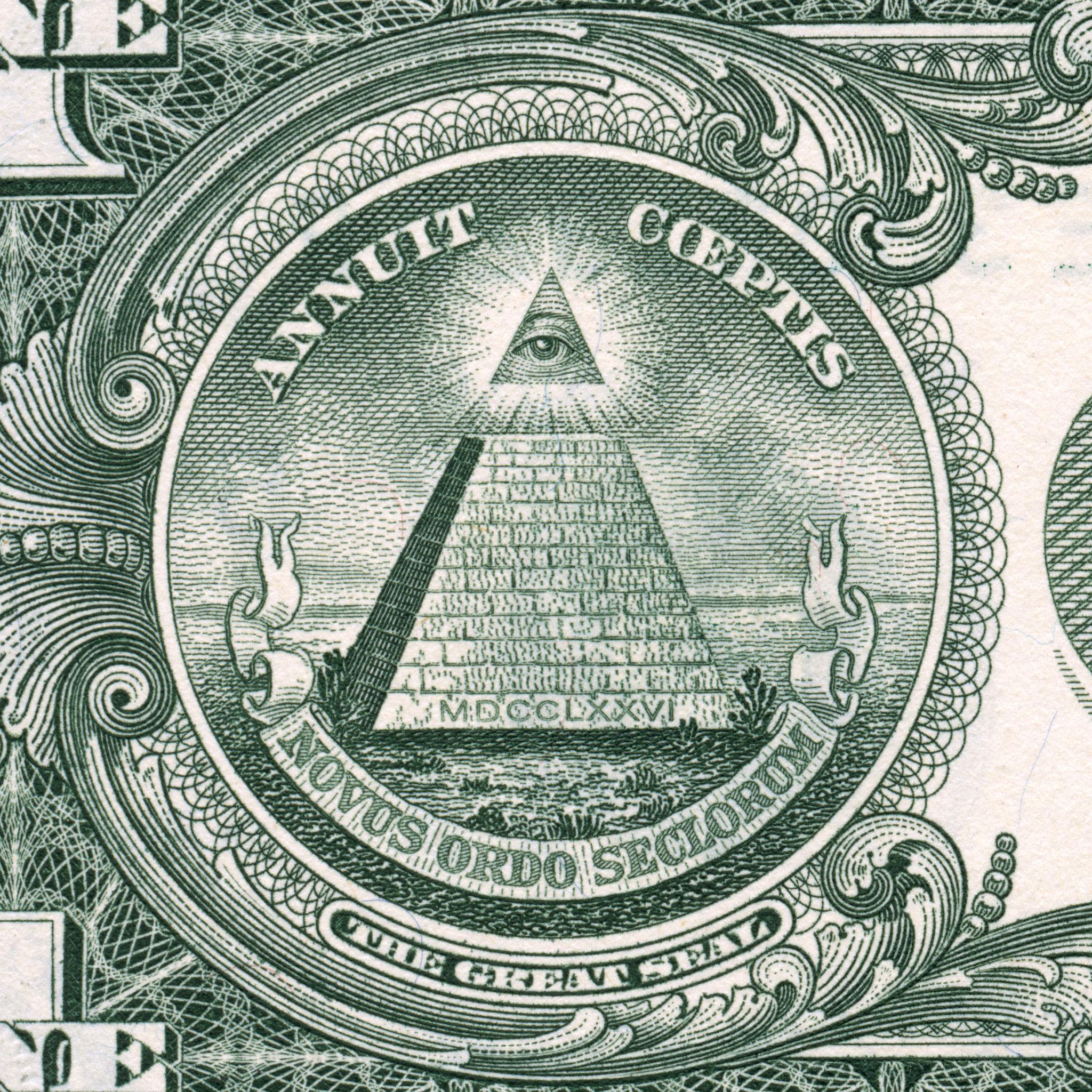
Just an image: an eye, a triangle, rays, an unfinished pyramid.
From that starting point, we:
- decomposed the symbol into observable parts
- grounded those parts in documented history
- separated structure from speculation
That produces a defensible analysis.
But it also exposes something more important:
the symbol is not a message, it is a composition.
That shift changed the problem.
We stopped asking:
What does this symbol mean?
And started asking:
What is it made of and can that structure be detected automatically?
To answer that, we built a working system:
- detect symbolic primitives
- represent them in a shared form (emoji)
- compare symbols by structure
- encode them into a searchable surface (ZeroModel)
This is not an interpretation engine.
It is a structure engine.
The result is simple: symbols can now be decomposed, compared, and searched without assuming meaning.
1. Solving the Symbol
The Eye of Providence first appeared as a promising test case for symbolic analysis. Its persistence, recognizability, and reputation for hidden meaning made it a natural candidate for experimentation.
The historical record, however, is more explicit than expected. Documentation around the Great Seal describes the major elements of the symbol in clear terms:
- an eye, enclosed in a triangle
- surrounded by rays of light
- positioned above an unfinished pyramid
- accompanied by a date marking the founding period
The structure also developed over time. Early versions included the Eye without the pyramid, indicating that the final composition was assembled rather than discovered as a single unit.
This detail changes how the symbol should be approached.
Instead of treating it as a fixed image with a single meaning, it is more useful to treat it as a constructed arrangement of parts.
Each component carries a recognizable role:
- the eye: observation or providence
- the triangle: enclosure or structure
- the rays: illumination or influence
- the pyramid: a layered system or foundation
- the spatial separation: perspective or external vantage
These elements combine into a coherent whole, but they remain separable. Their roles are stable even when the composition changes.
At that point, the central question shifts. Interpretation becomes less important than structure.
What matters is not what the symbol means, but how it is built and where those same components appear elsewhere.
That shift from meaning to composition is what makes the system in the next sections possible.
2. Symbols Are Compositions
The structure identified in the previous section suggests a different way to think about symbols.
The Eye of Providence does not behave like a single object with a fixed meaning. It behaves like a composition built from smaller, reusable elements. Those elements retain their roles even when the surrounding image changes.
This observation can be made concrete by isolating the components already identified:
| Primitive | Role |
|---|---|
| 👁️ Eye | observation / perception |
| 🔺 Triangle | enclosure / structure |
| ✨ Rays | illumination / influence |
| 🏛️ Pyramid | layered system / foundation |
| ⬆️ Above | external perspective / separation |
These primitives are not interpretations in the abstract sense. They are functional roles inferred from visible structure and documented context. Each can appear independently or in combination with others.
Once expressed in this form, comparison becomes straightforward.
The Eye of Providence can be represented as:
👁️ 🔺 ✨ 🏛️ ⬆️
A related symbol, such as a Masonic eye variant, typically resolves to a subset:
👁️ ✨ ⬆️
The overlap is explicit. Three primitives are shared. Two are absent. The relationship between the symbols can be described in structural terms rather than narrative ones.
This representation makes it possible to compare symbols without relying on surface appearance. Similarity emerges from shared components, not visual likeness alone.
The choice of emoji as a representation layer is practical rather than theoretical.
Emoji provide:
- discrete, visually distinct tokens
- a shared vocabulary that requires no additional training
- enough semantic weight to act as stand-ins for symbolic roles
Other representations are possible. Embedding vectors or custom ontologies could serve the same purpose with greater precision. Emoji are sufficient to demonstrate the underlying idea while remaining inspectable and easy to manipulate.
The key property is not the specific symbols used, but the existence of a shared intermediate form.
Once a symbol can be decomposed into primitives and expressed in that form, it can be:
- compared against other symbols
- clustered by structural similarity
- indexed for retrieval
At that point, the problem shifts again.
The task is no longer limited to explaining a single symbol. It becomes a question of identifying recurring structures across many symbols and measuring how those structures vary.
That transition leads directly into the implementation.
3. The Representation Layer
At this point we have primitives.
The remaining problem is not conceptual, it is technical.
How do we encode these primitives so they can be stored, compared, and searched?
The representation must satisfy four constraints:
- Discrete: each element should be clearly separable
- Composable: combinations should preserve structure
- Comparable: similarity should be measurable
- Inspectable: the output should remain understandable without additional tooling
The primitive set already provides structure. What remains is a way to encode it consistently.
Emoji provide a workable solution. Emoji are used here as compact symbolic tokens: inspectable by humans, comparable by machines, and sufficient for a first intermediate representation.
Each primitive can be mapped to a token:
- 👁️ → eye
- 🔺 → triangle
- ✨ → rays
- 🏛️ → pyramid
- ⬆️ → above
A symbol then becomes a sequence of tokens rather than a single image.
For example:
👁️ 🔺 ✨ 🏛️ ⬆️
This sequence captures the presence of components, but not yet their strength or relative importance. That information is preserved earlier in the pipeline as scores.
A more complete representation combines both:
eye=0.91, triangle=0.88, rays=0.72, pyramid=0.95, above=0.63
→ 👁️ 🔺 ✨ 🏛️ ⬆️
The numeric layer retains precision. The emoji layer provides a simplified view suitable for comparison and inspection.
This separation is intentional.
- The score vector acts as the underlying data
- The emoji sequence acts as a readable projection
The system operates on the scores. The emoji make the output usable.
At this stage, two symbols can be compared directly by evaluating overlap in their primitive sets. A simple measure such as intersection over union is sufficient to establish similarity.
For example:
A: 👁️ 🔺 ✨ 🏛️ ⬆️
B: 👁️ ✨ ⬆️

overlap = 3 / 5
This produces a structural similarity score without requiring any interpretation of meaning.
The same approach extends beyond images.
Any input that can be reduced to a set of primitives can be mapped into the same representation. The primitives themselves may differ by modality, but the encoding layer remains consistent.
- text → semantic roles
- video → actions and interactions
- audio → tempo and intensity patterns
The representation does not depend on the source. It depends only on the ability to extract a stable set of components.
At that point, the system gains a useful property.
Different types of data can be compared within a shared space, as long as they resolve to compatible primitives. The representation acts as a bridge between modalities.
This is sufficient for a prototype.
The goal is not to define a complete symbolic language. The goal is to establish a minimal intermediate form that supports decomposition, comparison, and extension.
With that in place, the next step is to show that the primitives can be extracted in practice.
This is the key transition.
The system does not treat symbols as labels.
It treats them as distributions over structure.
That changes what comparison means.
Two symbols no longer need to match exactly. They only need to share enough structure to overlap.
Similarity becomes a matter of shared composition, not identical identity.
This is what allows symbols to be compared, clustered, and searched without requiring a single “correct” interpretation.
4. Building the Prototype
At this point, the system is defined. This section demonstrates that the structure can be implemented.
The prototype takes an image as input and produces a set of primitive scores, along with a corresponding symbolic representation. The implementation relies on classical computer vision techniques rather than pretrained models. This keeps the process transparent and allows each step to be inspected.
The pipeline follows a fixed sequence:
-
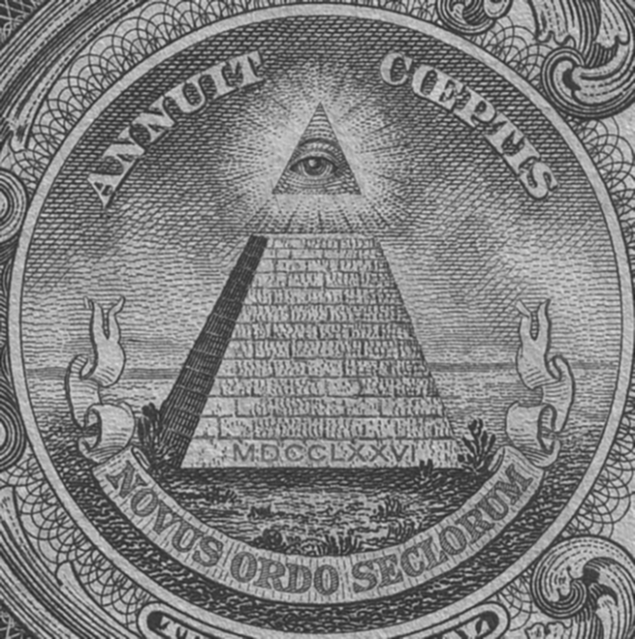
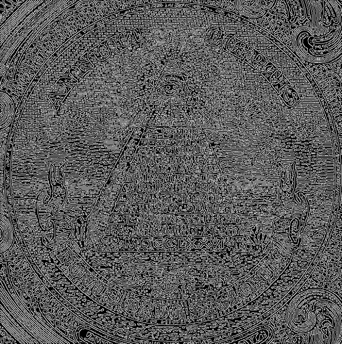
Preprocessing The image is converted to grayscale and normalized. Edge detection is applied to highlight structural boundaries.
-
Contour Extraction Contours are identified from the edge map. These serve as candidates for geometric primitives.
-
Shape Approximation Each contour is approximated to a geometric form:
- ellipses suggest the presence of an eye
- triangles suggest enclosure or structure
- radial patterns suggest rays
-
Spatial Analysis The relative positions of detected shapes are evaluated:
- vertical separation indicates “above”
- central alignment increases confidence in composite structures
-
Scoring Each primitive is assigned a score based on detection confidence and spatial consistency. The result is a vector of primitive strengths.
A typical output from this process looks like this:
{
  "eye": 0.91,
  "triangle": 0.88,
  "rays": 0.72,
  "pyramid": 0.95,
  "above": 0.63
}
This vector is the primary output of the system. It captures the structural composition of the image in a form that can be compared numerically.
The emoji representation is derived from this vector:
👁️ 🔺 ✨ 🏛️ ⬆️
The prototype was evaluated against a small test set to validate behavior across different inputs.
Examples:
eye_symbol_1:
detected: ['triangle', 'eye', 'rays', 'above', 'sun']
expected: ['triangle', 'eye', 'rays']
precision: 0.6, recall: 1.0

star:
detected: ['sun', 'eye', 'star', 'rays']
expected: ['star']
precision: 0.25, recall: 1.0

tree:
detected: ['eye', 'tree', 'rays']
expected: ['tree']
precision: 0.33, recall: 1.0
The results show a consistent pattern.
Recall remains high across cases. The system detects relevant primitives reliably. Precision is lower, particularly where primitives overlap conceptually. For example, stars and suns both trigger radial and brightness-based features, leading to shared detections.
This behavior is expected.
The prototype does not enforce strict classification. It identifies structural features and assigns them to multiple primitives when appropriate. Overlap is preserved rather than suppressed.
This allows the output to reflect ambiguity present in the input, rather than forcing a single label.
At this stage, the system satisfies the core requirement:
- primitives can be detected from real images
- detections can be expressed as structured scores
- scores can be converted into a shared representation
This is sufficient to move beyond individual symbols.
The next step is to examine how overlapping detections affect comparison.
| Original | Grayscale | Edges | Contours |
|---|---|---|---|
 |
 |
 |
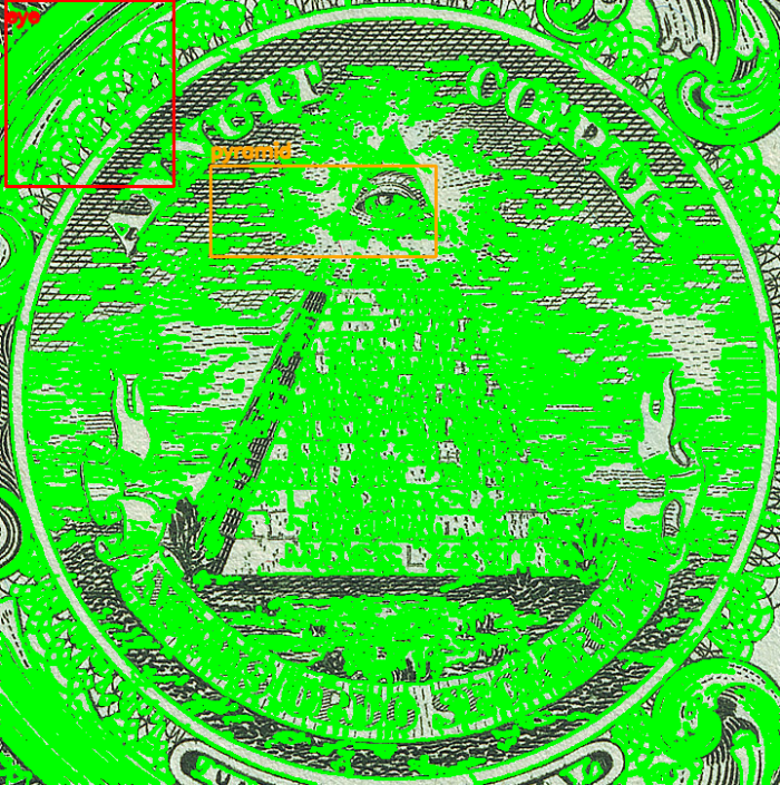 |
Figure 1 — From Image to Symbolic Signature
The implementation can be summarized as a short symbolic pipeline: structural and semantic signals are merged into primitives, then projected into a shared representation.
    %%{init: {
  'theme': 'base',
  'themeVariables': {
    'primaryColor': '#e3f2fd',
    'primaryTextColor': '#0d2135',
    'primaryBorderColor': '#1e88e5',
    'lineColor': '#1565c0',
    'secondaryColor': '#bbdefb',
    'tertiaryColor': '#90caf9',
    'background': '#f0f8ff',
    'mainBkg': '#e3f2fd',
    'textColor': '#0d2135'
  },
  'flowchart': {
    'curve': 'basis',
    'padding': 20
  }
}}%%

graph TB
    subgraph Input["🖼️ INPUT"]
        A[("📷 Image<br><small>Eye of Providence</small>")]
        style A fill:#42a5f5,stroke:#1565c0,stroke-width:3px,color:#fff
    end

    subgraph Detection["🔍 DETECTION LAYER"]
        direction TB
        B1["🧠 CLIP<br><small>Semantic Scoring</small>"]
        B2["👁️ CV2<br><small>Structural Features</small>"]
        style B1 fill:#7e57c2,stroke:#4527a0,stroke-width:2px,color:#fff
        style B2 fill:#7e57c2,stroke:#4527a0,stroke-width:2px,color:#fff
    end

    subgraph Primitives["🧩 PRIMITIVE EXTRACTION"]
        direction LR
        C1["👁️ Eye<br><small>0.91</small>"]
        C2["🔺 Triangle<br><small>0.88</small>"]
        C3["✨ Rays<br><small>0.72</small>"]
        C4["🏛️ Pyramid<br><small>0.95</small>"]
        C5["⬆️ Above<br><small>0.63</small>"]
        style C1 fill:#26c6da,stroke:#00695c,stroke-width:2px,color:#fff
        style C2 fill:#26c6da,stroke:#00695c,stroke-width:2px,color:#fff
        style C3 fill:#26c6da,stroke:#00695c,stroke-width:2px,color:#fff
        style C4 fill:#26c6da,stroke:#00695c,stroke-width:2px,color:#fff
        style C5 fill:#26c6da,stroke:#00695c,stroke-width:2px,color:#fff
    end

    subgraph Graph["🕸️ SYMBOLIC GRAPH"]
        direction TB
        D1["🔺 contains 👁️"]
        D2["👁️ emits ✨"]
        D3["👁️ above 🏛️"]
        style D1 fill:#ffa726,stroke:#e65100,stroke-width:2px,color:#0d2135
        style D2 fill:#ffa726,stroke:#e65100,stroke-width:2px,color:#0d2135
        style D3 fill:#ffa726,stroke:#e65100,stroke-width:2px,color:#0d2135
    end

    subgraph IR["🔤 INTERMEDIATE REPRESENTATION"]
        E["👁️ 🔺 ✨ 🏛️ ⬆️<br><small>Emoji Sequence</small>"]
        style E fill:#ef5350,stroke:#b71c1c,stroke-width:3px,color:#fff
    end

    subgraph ZeroModel["🗺️ ZEROMODEL INDEXING"]
        direction LR
        F1["📊 Score Matrix"]
        F2["🖼️ PNG Surface"]
        F3["🧭 Spatial Navigation"]
        style F1 fill:#66bb6a,stroke:#1b5e20,stroke-width:2px,color:#fff
        style F2 fill:#66bb6a,stroke:#1b5e20,stroke-width:2px,color:#fff
        style F3 fill:#66bb6a,stroke:#1b5e20,stroke-width:2px,color:#fff
    end

    subgraph Output["🎯 OUTPUT"]
        G["🔎 Similar Symbols<br><small>Masonic Eye, Sun, Star...</small>"]
        style G fill:#42a5f5,stroke:#1565c0,stroke-width:3px,color:#fff
    end

    A --> B1
    A --> B2
    B1 --> C1
    B1 --> C2
    B1 --> C3
    B1 --> C4
    B2 --> C1
    B2 --> C2
    B2 --> C3
    B2 --> C4
    B2 --> C5

    C1 --> D1
    C2 --> D1
    C1 --> D2
    C3 --> D2
    C1 --> D3
    C4 --> D3
    C5 --> D3

    D1 --> E
    D2 --> E
    D3 --> E

    E --> F1
    F1 --> F2
    F2 --> F3
    F3 --> G

    %% Subgraph styling
    style Input fill:#e3f2fd,stroke:#1e88e5,stroke-width:2px
    style Detection fill:#ede7f6,stroke:#4527a0,stroke-width:2px
    style Primitives fill:#e0f7fa,stroke:#00695c,stroke-width:2px
    style Graph fill:#fff3e0,stroke:#e65100,stroke-width:2px
    style IR fill:#ffebee,stroke:#b71c1c,stroke-width:2px
    style ZeroModel fill:#e8f5e9,stroke:#1b5e20,stroke-width:2px
    style Output fill:#e3f2fd,stroke:#1565c0,stroke-width:2px
The original image is progressively transformed into grayscale, edge maps, and contour overlays to expose its underlying geometry. Each stage removes visual noise while preserving structure, making implicit shapes explicit.
This sequence shows how the system moves from appearance to measurable structure—the foundation for all later symbolic detection.
A Concrete Example From Image to Structure
To make the pipeline explicit, we can trace a single image all the way through the system.
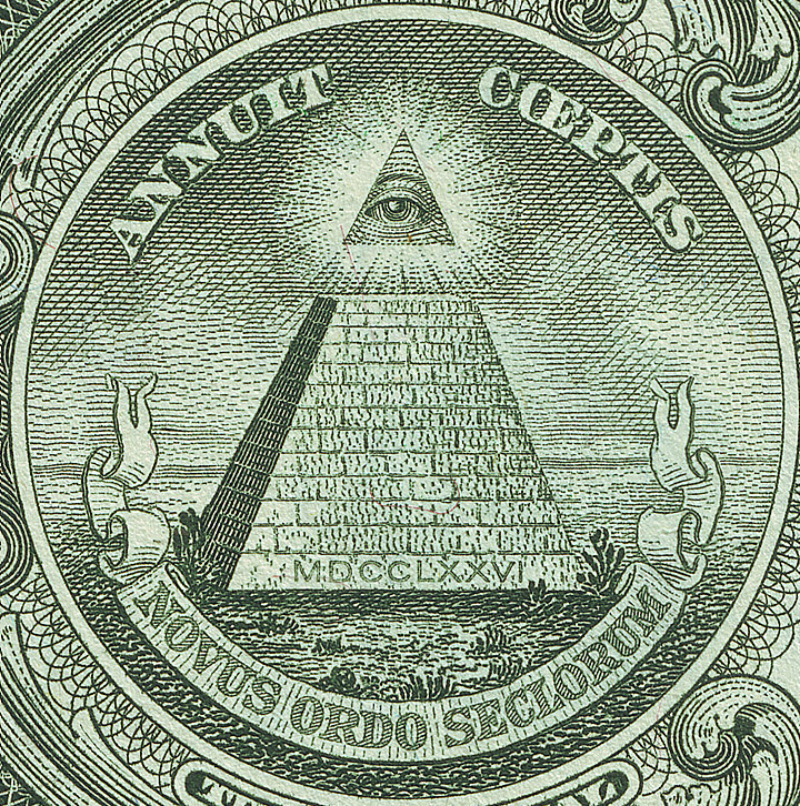
Input
Eye of Providence (Great Seal variant)
Step 1 Structural Extraction (CV2)
The image is transformed through a sequence of structural filters:
| Stage | Output Description |
|---|---|
| Grayscale | Normalized intensity, removes color noise |
| Edges | Canny edge map highlights boundaries |
| Contours | Geometric shapes extracted from edges |
At this stage, the system is not identifying meaning, it is identifying geometry and structure.
From these signals, candidate primitives emerge:
- elliptical contour → potential eye
- triangular contour → potential triangle
- radial edge dispersion → potential rays
- lower mass region → potential pyramid
Step 2 Semantic Scoring (CLIP)
In parallel, the image is compared against primitive concepts:
"eye", "triangle", "rays", "pyramid", "above"
This produces similarity scores based on learned visual-language alignment.
Step 3 Combined Primitive Scores
The structural and semantic signals are combined:
eye       = 0.91
triangle  = 0.88
rays      = 0.72
pyramid   = 0.95
above     = 0.63
This is the core representation of the image.
Not a label. Not a classification.
A distribution of symbolic primitives.
Step 4 Graph Construction
The system then evaluates relationships between primitives:
triangle → contains → eye
eye      → emits    → rays
eye      → above    → pyramid
This converts the flat vector into a structured symbolic graph.
Step 5 Intermediate Representation
The graph is projected into the shared symbolic layer:
👁️ 🔺 ✨ 🏛️ ⬆️
This is not decoration.
It is a compressed, comparable encoding of structure.
Step 6 Comparison Against Another Symbol
Now consider a related image:
Masonic Eye Variant
The system produces:
eye       = 0.84
rays      = 0.69
above     = 0.71
triangle  = 0.12
pyramid   = 0.08

→ 👁️ ✨ ⬆️
Step 7 Structural Similarity
We can now compare the two symbols:
A: 👁️ 🔺 ✨ 🏛️ ⬆️
B: 👁️ ✨ ⬆️

Overlap: 3 / 5 primitives
This establishes similarity without relying on visual matching.
The images differ in appearance, but share structural components.
What This Demonstrates
This example shows the full pipeline:
- Image → structural features
- Features → primitive scores
- Scores → symbolic graph
- Graph → intermediate representation
- Representation → comparable structure
The system does not decode meaning.
It extracts structure and makes that structure measurable.
5. Symbolic Overlap
The prototype does not produce clean, mutually exclusive labels. A single image often activates multiple primitives at once, even when only one was expected.
This is visible in the evaluation results:
star:
detected: ['sun', 'eye', 'star', 'rays']

sun:
detected: ['eye', 'halo', 'sun', 'star', 'above', 'rays']
At first glance, this looks like reduced precision. A star should not necessarily be a sun. A sun should not necessarily include an eye.
That interpretation assumes that primitives are exclusive categories. The prototype shows that they are not.
The detection process operates on structural features:
- radial symmetry
- brightness gradients
- central focus
- contour density
These features are shared across multiple symbolic interpretations. A sun and a star both exhibit radial structure. Rays of light appear in both cases. The system responds to those shared signals.
As a result, the output is not a single label. It is a set of overlapping activations.
This behavior is consistent across other examples:
tree:
detected: ['eye', 'tree', 'rays']

eagle:
detected: ['eagle', 'eye', 'above', 'rays']
The additional primitives are not random. They correspond to partial structural matches:
- “eye” can be triggered by elliptical regions or high-contrast focal points
- “rays” can be triggered by directional edge patterns
- “above” can be triggered by vertical separation
The system is capturing fragments of structure rather than enforcing a single interpretation.
This leads to a different way of reading the output.
Instead of asking which label is correct, it becomes more useful to ask:
- which primitives are strongly activated
- which primitives co-occur
- how the activation pattern compares to other inputs
A symbol can then be represented as a signature, not a classification.
For example:
Eye of Providence:
[eye, triangle, rays, pyramid, above]

Masonic variant:
[eye, rays, above]

Star:
[star, rays, sun]

Sun:
[sun, rays, star, above]
These signatures overlap in structured ways. Similar symbols share subsets of primitives. Dissimilar symbols diverge.
This has two immediate consequences.
First, similarity becomes a matter of degree, not identity. Two symbols do not need to match exactly to be related. Shared structure is sufficient.
Second, ambiguity is preserved rather than removed. The system does not force a decision between “sun” and “star” when both are supported by the data.
This behavior is closer to how continuous representations operate in embedding models. Multiple related concepts occupy nearby regions and can be activated together. The difference here is that the representation remains explicit and interpretable.
The prototype therefore establishes an important property:
Symbolic meaning is not exclusive. It is compositional and overlapping.
This property becomes useful in the next step.
If symbols can be represented as overlapping sets of primitives, then those sets can be encoded, stored, and compared at scale.
Example Results: Symbolic Overlap in Practice
The table shows detected primitives compared to expected ones across multiple images. While recall remains high, precision varies due to overlapping structural features shared between symbols.
This illustrates that symbols are not exclusive categories but compositional structures with shared components.
| Image | Expected Symbols | Detected Symbols | Precision | Recall |
|---|---|---|---|---|
| Eye #1 | rays, eye, triangle | above, triangle, rays, eye, sun | 0.60 | 1.00 |
| Eye #2 | rays, eye, triangle | above, triangle, rays, eye, sun | 0.60 | 1.00 |
| Eye #3 | rays, eye, triangle | star, above, rays, triangle, eye, sun | 0.50 | 1.00 |
| Star | star | star, sun, eye, rays | 0.25 | 1.00 |
| Sun | sun, rays | star, above, rays, eye, sun, halo | 0.33 | 1.00 |
| Tree | tree | tree, eye, rays | 0.33 | 1.00 |
| Eagle | eagle | eagle, above, eye, rays | 0.25 | 1.00 |
| Landscape | above, tree, eye, rays | 0.00 | 0.00 | |
| Dog | above, eye, rays | 0.00 | 0.00 |
The system treats symbols as distributions over structure. That is what makes comparison possible even when identity is ambiguous.
6. ZeroModel: From Symbols to Searchable Structure
Up to this point, we have a working pipeline:
- an image goes in
- primitives are detected
- the result is a structured set of scores
For example:
eye       = 0.91
triangle  = 0.88
rays      = 0.72
pyramid   = 0.95
above     = 0.63
This is already useful. It tells us what structures are present.
But it is not yet scalable.
We cannot compare millions of these objects efficiently by looping through vectors. We need a representation that is compact, indexable, and fast to query.
That is where ZeroModel enters.
The Core Idea
ZeroModel does something very simple:
It takes a matrix of primitive scores and encodes it into an image.
That’s it.
- Each row represents an item (an image, a document, a scene)
- Each column represents a primitive or metric
- Each value is encoded as an intensity
The result is a dense visual structure typically stored as a PNG.
This is not just a visualization.
It is the data structure itself.
The same representation that can be inspected visually is also the structure the system operates on.
From Vectors to a Surface
Instead of storing:
[0.91, 0.88, 0.72, 0.95, 0.63, ...]
we encode it as:
- pixel intensity
- spatial position
- channel value (if needed)
So a dataset becomes:
- a 2D grid of rows (items)
- a wide axis of columns (primitives)
- intensity representing strength
At small scale, this looks like an image.
At large scale, it becomes a structured surface of meaning.
Why This Matters
Once the data is encoded this way, something changes.
We are no longer working with:
- lists
- dictionaries
- embeddings in isolation
We are working with a spatially organized representation.
That enables:
- fast slicing (rows, columns, regions)
- locality-based search
- hardware-accelerated operations (image-level ops)
In other words:
We can navigate structure instead of scanning data.
Once structure is spatial, similarity becomes distance.
The Important Constraint
ZeroModel only works because of what came before it.
If the primitives were noisy or inconsistent, the encoding would collapse into randomness.
But because:
- primitives are reusable
- scores are comparable
- overlap is meaningful
the encoded surface retains structure.
Clusters form naturally.
Similar items appear near each other.
Outliers stand out immediately.
What This Gives Us
With this representation, we can:
- Store large numbers of symbolic decompositions compactly
- Compare items by spatial proximity instead of pairwise computation
- Build indexes that operate on structure instead of raw data
- Query patterns directly (e.g. “high eye + high rays + above”)
This is the first point where the system stops being a prototype and starts becoming infrastructure.
A Concrete Way to Think About It
Think of ZeroModel like this:
Instead of searching through a library book by book, you build a map of the entire library.
You don’t ask:
“Does this book match?”
You ask:
“Where on the map do similar books live?”
The PNG is that map.
Another way to understand this is in terms of resonance.
Because all items are encoded into the same surface, a query does not search the dataset.
It resonates with it.
The query activates regions where its structure is already present.
Similarity is not computed from scratch.
It emerges from where the structure “vibrates” most strongly on the surface.
What It Is Not
It is not:
- a trained model
- a neural network
- a learned embedding space
It does not learn weights.
It preserves structure.
That is why we call it ZeroModel.
Where This Leads
Once primitive scores can be encoded into a shared surface:
- images can be compared to images
- images can be compared to text (via the same primitives)
- patterns can be detected across large datasets
And crucially:
search becomes navigation.
That transition from comparison to navigation is what makes the next step possible.
7. Indexing: From Storage to Navigation
Once primitive scores are encoded into a ZeroModel surface, the problem changes.
We are no longer asking how to store data.
We are asking:
How do we move through it?
The Shift
In a traditional system, search looks like this:
- take a query
- compare it against every item
- rank the results
Even with optimizations, this is still a form of scanning.
ZeroModel allows a different approach.
Because the data is already organized spatially, we can treat it as something to navigate.
The Structure
The encoded surface is not just a flat image.
It is organized:
- rows represent items
- columns represent primitives
- regions represent clusters of similar structure
This gives us a natural hierarchy.
At a high level:
- broad regions correspond to coarse patterns
- smaller regions refine those patterns
- individual rows represent specific items
So instead of searching linearly, we move:
- from large regions
- into smaller regions
- down to specific matches
How a Query Works
A query in this system is just another set of primitive scores.
For example:
eye       = high
rays      = high
triangle  = medium
above     = present
This can be encoded in the same way as the dataset.
Once encoded, the query becomes a position on the surface.
Search becomes:
- locate the region that matches the query pattern
- move toward areas of higher similarity
- retrieve nearby items
There is no need to compare against every row.
We move directly to the relevant area.
Why This Is Fast
The speed comes from two properties:
1. Locality
Similar structures are stored near each other.
That means:
- you don’t need global comparisons
- you only explore a small region
2. Fixed Representation
Everything is already encoded in the same format.
There is no transformation step at query time.
The system is always “ready to search.”
What This Enables
With indexing in place, we can:
- retrieve structurally similar symbols instantly
- cluster large datasets by primitive composition
- explore variations of a pattern without predefined labels
- detect outliers as regions with low density
More importantly:
we can search for structure directly.
Not keywords. Not labels. Not categories.
Structure.
A Simple Example
If we query for:
- strong eye
- strong rays
- clear separation (above)
we land in the region containing:
- Eye of Providence variants
- Masonic eye symbols
- other “observer + illumination” structures
Even if the images look different at the surface level, they cluster together because their primitives align.
The Practical Outcome
At this point, the system has three properties:
- Decomposition complex inputs become primitives
- Representation primitives become a shared surface
- Indexing the surface becomes navigable
That combination is what allows the system to scale.
The Key Transition
Before this point, we were analyzing individual symbols.
After this point, we can explore entire datasets.
That is the transition:
from understanding one symbol to navigating symbolic structure at scale
Where This Leads
Once navigation is possible:
- we can search across images
- extend the same primitives to text
- eventually unify multiple modalities
The system is no longer tied to a single input type.
It operates on structure.
8. The Bigger Question: Why Do These Patterns Persist?
Up to this point, we have stayed grounded in what we can measure:
- symbols can be decomposed into primitives
- those primitives can be detected across images
- different symbols share overlapping structure
- that structure can be encoded and indexed
That is the system.
What remains is the question that motivated it.
The Observation
Certain symbols appear again and again:
- the eye
- the star
- the sun
- the eagle
- hierarchical structures
They persist across:
- cultures
- time periods
- mediums
These are not isolated occurrences.
They are recurring patterns.
What We Can Now Say (Carefully)
Before this work, we could only describe that persistence.
Now we can begin to measure it.
We can:
- extract primitives from large sets of images
- compare their structure
- cluster symbols by similarity
- track how those clusters appear over time
This turns a qualitative observation into a quantitative one.
What This Changes
Before this system, symbolic analysis had two modes:
- manual interpretation (subjective, slow)
- visual similarity (fragile, surface-level)
This introduces a third:
structural comparison
Symbols can now be compared based on what they are made of, not how they look or how they are described.
That makes new types of analysis possible:
- tracking primitive frequency across datasets
- identifying recurring structural patterns
- clustering symbols without predefined labels
This does not answer why symbols persist.
But it makes that question measurable.
The Hypothesis
A reasonable hypothesis emerges:
Persistent symbols are composed of reusable structural primitives, and those primitives reflect recurring patterns in how humans represent ideas.
This does not claim hidden meaning.
It does not require conspiracy.
It only requires that:
- humans reuse structures that work
- those structures become stable over time
Why This Matters
If symbolic structure can be measured, then it can be studied.
For example:
- Do certain primitives appear more frequently in specific eras?
- Do clusters of symbols shift during periods of change?
- Do different cultures converge on similar structures independently?
These questions were previously difficult to approach in a systematic way.
Now they are at least technically feasible.
The Important Boundary
This system does not interpret symbols.
It does not assign meaning.
It identifies structure.
Any interpretation comes after.
Where This Leads
The immediate application is clear:
- large-scale symbolic analysis
- structural comparison across datasets
- discovery of related forms without predefined labels
Beyond that, there is a broader direction:
using structure as a lens to study human expression.
That includes:
- images
- text
- eventually video and audio
The system does not depend on the medium.
It depends on decomposition and representation.
The Position We Take
We are not claiming to explain why these symbols exist.
We are claiming something more modest and more useful:
we now have a way to detect and compare the structures that make them persist.
That is enough to move forward.
Figure 2: Full System Architecture
By this point, the Eye of Providence is only the entry point. The broader system can be understood as a general pipeline for extracting, representing, comparing, and indexing symbolic structure across modalities
%%{init: {
  'theme': 'base',
  'themeVariables': {
    'primaryColor': '#e3f2fd',
    'primaryTextColor': '#0d2135',
    'primaryBorderColor': '#1e88e5',
    'lineColor': '#1565c0',
    'secondaryColor': '#bbdefb',
    'tertiaryColor': '#90caf9',
    'background': '#f0f8ff',
    'mainBkg': '#e3f2fd',
    'textColor': '#0d2135'
  },
  'flowchart': {
    'curve': 'basis',
    'padding': 20
  }
}}%%

flowchart TD
    subgraph Inputs["🌐 INPUT MODALITIES"]
        direction LR
        A1["🖼️ Images"]
        A2["📝 Text"]
        A3["🎬 Video"]
        A4["🎵 Audio / Music"]
        style A1 fill:#42a5f5,stroke:#1565c0,stroke-width:2px,color:#fff
        style A2 fill:#42a5f5,stroke:#1565c0,stroke-width:2px,color:#fff
        style A3 fill:#42a5f5,stroke:#1565c0,stroke-width:2px,color:#fff
        style A4 fill:#42a5f5,stroke:#1565c0,stroke-width:2px,color:#fff
    end

    subgraph Detection["🔍 PRIMITIVE DETECTION LAYER"]
        B["🧩 Extract Primitives<br><small>CV2 + CLIP / Semantic + Structural</small>"]
        style B fill:#7e57c2,stroke:#4527a0,stroke-width:2px,color:#fff
    end

    A1 --> B
    A2 --> B
    A3 --> B
    A4 --> B

    subgraph Scores["📊 PRIMITIVE SCORE VECTORS"]
        C["👁️ 0.91  🔺 0.88  ✨ 0.72  🏛️ 0.95  ⬆️ 0.63 ..."]
        style C fill:#26c6da,stroke:#00695c,stroke-width:2px,color:#fff
    end

    B --> C

    C --> D["🔤 Intermediate Representation<br/><small>Emoji / Symbolic Tokens</small>"]
    style D fill:#ef5350,stroke:#b71c1c,stroke-width:3px,color:#fff

    C --> E["🕸️ Symbol Graph Construction"]
    style E fill:#ffa726,stroke:#e65100,stroke-width:2px,color:#0d2135

    subgraph GraphAnalysis["🧠 GRAPH ANALYSIS"]
        direction LR
        F["📐 Graph Similarity"]
        G["🔬 Invariant Extraction"]
        H["🧬 Clustering"]
        style F fill:#66bb6a,stroke:#1b5e20,stroke-width:2px,color:#fff
        style G fill:#66bb6a,stroke:#1b5e20,stroke-width:2px,color:#fff
        style H fill:#66bb6a,stroke:#1b5e20,stroke-width:2px,color:#fff
    end

    E --> F
    E --> G
    E --> H

    subgraph Shared["🤝 SHARED SYMBOLIC SIGNATURE"]
        I["👁️ 🔺 ✨ 🏛️ ⬆️"]
        style I fill:#ab47bc,stroke:#6a1b9a,stroke-width:3px,color:#fff
    end

    D --> I
    F --> I
    G --> I
    H --> I

    subgraph ZeroModel["🗺️ ZEROMODEL ENCODING"]
        direction LR
        J["📊 Score Matrix"]
        K["🖼️ PNG Surface"]
        L["🧭 Spatial Navigation"]
        style J fill:#8d6e63,stroke:#4e342e,stroke-width:2px,color:#fff
        style K fill:#8d6e63,stroke:#4e342e,stroke-width:2px,color:#fff
        style L fill:#8d6e63,stroke:#4e342e,stroke-width:2px,color:#fff
    end

    I --> J
    J --> K
    K --> L

    subgraph Search["🔎 SEARCH & RETRIEVAL"]
        direction LR
        M["🧱 Structure Search"]
        N["🔍 Pattern Retrieval"]
        O["🔁 Cross‑Modal Comparison"]
        style M fill:#42a5f5,stroke:#1565c0,stroke-width:2px,color:#fff
        style N fill:#42a5f5,stroke:#1565c0,stroke-width:2px,color:#fff
        style O fill:#42a5f5,stroke:#1565c0,stroke-width:2px,color:#fff
    end

    L --> M
    L --> N
    L --> O

    O --> P["💡 Research Direction<br/><small>persistent symbolic structure<br/>across human expression</small>"]
    style P fill:#e3f2fd,stroke:#1e88e5,stroke-width:3px,color:#0d2135

    %% Subgraph backgrounds
    style Inputs fill:#e3f2fd,stroke:#1e88e5,stroke-width:2px
    style Detection fill:#ede7f6,stroke:#4527a0,stroke-width:2px
    style Scores fill:#e0f7fa,stroke:#00695c,stroke-width:2px
    style GraphAnalysis fill:#e8f5e9,stroke:#1b5e20,stroke-width:2px
    style Shared fill:#f3e5f5,stroke:#6a1b9a,stroke-width:2px
    style ZeroModel fill:#efebe9,stroke:#4e342e,stroke-width:2px
    style Search fill:#e3f2fd,stroke:#1565c0,stroke-width:2px
A single image is processed through structural extraction, semantic scoring, graph construction, and symbolic projection. The result is a compact representation of the image as a set of primitives and relationships.
This demonstrates that symbolic structure can be derived directly from visual input without requiring predefined labels.
8.5 A Symbolic Weather Station
If symbolic structure can be measured, then it can also be tracked.
Across time. Across datasets. Across cultures.
This suggests a different kind of system:
a symbolic weather station.
Instead of measuring temperature or pressure, it measures:
- primitive frequency
- structural overlap
- symbolic density
Spikes in certain primitives or patterns may indicate shifts in:
- cultural focus
- collective attention
- representation of authority or perception
This is not interpretation.
It is measurement.
But it creates the conditions for something new:
the ability to observe how symbolic structure evolves over time.
9. Conclusion: From One Symbol to a System
We started with a single image.
A symbol that appears on a dollar bill. A symbol that has been discussed, interpreted, and debated for decades.
The original goal was simple:
use AI to understand what it meant.
What We Found
The historical answer exists.
The Eye of Providence is not an unsolved mystery. Its components are documented, its evolution is known, and its meaning at least in its original context is well understood.
That could have been the end of the investigation.
It wasn’t.
The Shift in Perspective
Once the symbol was broken down into its components, the problem changed.
Instead of asking:
“What does this symbol mean?”
we began asking:
“What is this symbol made of?”
That shift made the system possible.
What We Built
We built a pipeline that:
- extracts primitives from images
- represents them in a shared form
- compares symbols by structure
- encodes those structures into a searchable surface
- and navigates that surface efficiently
Each step is simple on its own.
Together, they form something new:
a way to work with symbolic structure directly.
What It Shows
The results are not perfect.
Precision is low in some cases. Symbols overlap. Different images share the same primitives.
But that behavior is consistent.
And more importantly, it is explainable.
The system is not guessing.
It is detecting structure.
What Changed
At the beginning, the symbol looked like something to decode.
By the end, it looks like something to decompose.
That difference matters.
Because once something can be decomposed:
- it can be compared
- it can be indexed
- it can be searched
- it can be studied at scale
What This Enables
The immediate use case is clear:
- finding structurally similar symbols
- clustering visual patterns
- exploring variation without predefined labels
Beyond that, the same approach can extend to:
- text
- video
- other forms of human expression
The system does not depend on the medium.
It depends on structure.
Where This Leaves Us
We did not set out to build a general system.
We set out to understand one symbol.
That constraint kept the problem grounded.
It also revealed something broader:
the method scales beyond the original question.
The Final Position
We are not claiming to have explained symbolic meaning.
We are claiming something simpler:
symbolic structure can be extracted, represented, and compared in a consistent way.
That is enough to move forward.
The Closing Line
We started with a symbol.
Something fixed. Something already interpreted.
We expected to explain it.
Instead, we decomposed it.
And once it could be decomposed:
- it could be compared
- it could be indexed
- it could be searched
The Eye of Providence was not the answer.
It was the first example.
The system is what we were actually building.
The Eye is not watching. It is the thing that made us start seeing structure.
The Recursive Observation
There is one final detail worth noting.
The symbol we chose to analyze is itself a representation of observation.
An eye, positioned above a structure, emitting rays.
A system that looks at a system.
That is exactly what this pipeline does.
It observes structure from above, decomposes it into components, and maps relationships between them.
In that sense, the Eye of Providence was not just a test case.
It was a blueprint.
We did not just analyze the symbol.
We built the mechanism it represents.
10. Methods
This section formalizes the system described in the post. The goal is to define the pipeline in precise, reproducible terms.
10.1 Problem Definition
Given an input \( x \) (image, text, video, or audio), we aim to compute a structured representation:
$$ x \rightarrow S(x) $$Where:
- \( S(x) \) is a symbolic signature
- composed of primitives \( p_i \in P \)
- each associated with a score \( s_i \in [0,1] \)
The objective is not classification, but decomposition into reusable structural components.
10.2 Primitive Space
Let \( P \) be a finite set of primitives:
$$ P = \{ \text{eye}, \text{triangle}, \text{rays}, \text{pyramid}, \text{above}, \dots \} $$Each primitive is defined by:
- a symbolic identity
- a detection interface
- optional aliases and configuration
Primitives are:
- reusable
- composable
- non-exclusive
10.3 Detection Function
We define a detection function:
$$ D(x, p_i) \rightarrow s_i $$Where:
- \( x \) is the input
- \( p_i \) is a primitive
- \( s_i \) is the confidence score
In the prototype, detection is hybrid:
$$ s_i = w_{cv2} \cdot s_i^{cv2} + w_{clip} \cdot s_i^{clip} $$Where:
- \( s_i^{cv2} \): structural score (edges, contours, geometry)
- \( s_i^{clip} \): semantic score (vision-language similarity)
10.4 Structural Representation
The primitive scores form a vector:
$$ \mathbf{s} = [s_1, s_2, \dots, s_n] $$This vector is interpreted as a distribution over structure, not a label.
10.5 Graph Construction
A symbolic graph \( G(x) \) is constructed:
$$ G(x) = (V, E) $$Where:
- \( V = \{p_i\} \) are primitives
- \( E \subseteq V \times R \times V \) are relations
Example relations:
- contains
- emits
- above
Edges are added based on thresholded scores and spatial constraints.
10.6 Intermediate Representation
A projection function maps primitives to tokens:
$$ \phi: P \rightarrow T $$Where \( T \) is a set of symbolic tokens (emoji in the prototype).
$$ S_{IR}(x) = \{ \phi(p_i) \mid s_i > \tau \} $$This produces a discrete, comparable representation.
10.7 Similarity Metric
Similarity between two inputs is computed over primitives or graph structure.
Primitive Overlap (Jaccard-style)
$$ \text{sim}(A, B) = \frac{|P_A \cap P_B|}{|P_A \cup P_B|} $$Graph Similarity
$$ \text{sim}(G_A, G_B) = \frac{\sum \min(w_A(e), w_B(e))}{|E_A \cup E_B|} $$This captures relational similarity, not just presence.
10.8 ZeroModel Encoding
Primitive score vectors are aggregated into a matrix:
$$ M \in \mathbb{R}^{N \times |P|} $$Where:
- \( N \) = number of inputs
- columns = primitives
The matrix is encoded as an image:
$$ M \rightarrow I_{png} $$Where:
- pixel intensity represents score magnitude
- spatial layout preserves structure
This creates a symbolic surface.
10.9 Search via Navigation
Given a query \( q \):
- compute \( S(q) \)
- encode into surface space
- locate region of highest similarity
Search becomes:
$$ q \rightarrow \text{position on surface} \rightarrow \text{local traversal} $$This replaces global comparison with localized navigation.
10.10 Summary
The full pipeline can be expressed as:
$$ x \rightarrow D(x) \rightarrow S(x) \rightarrow G(x) \rightarrow IR(x) \rightarrow Z(x) $$Where:
- \( D \): detection
- \( S \): symbolic signature
- \( G \): graph
- \( IR \): intermediate representation
- \( Z \): ZeroModel encoding
The system transforms raw input into structured, comparable, and navigable symbolic representations.
11. Limitations and Future Work
The system described in this post is a working prototype. While it demonstrates the feasibility of symbolic decomposition and structural comparison, it has important limitations.
11.1 Limited Primitive Vocabulary
The current system operates on a small, manually defined set of primitives.
Limitations:
- incomplete coverage of symbolic space
- bias toward predefined structures
- limited generalization
Future Work:
- automatic primitive discovery from data
- hierarchical primitive taxonomies
- dynamic expansion of symbolic vocabulary
11.2 Detection Noise and Overlap
The system intentionally preserves overlapping detections.
Limitations:
- reduced precision
- ambiguous outputs
- sensitivity to shared structural features
While this behavior reflects compositional structure, it can make downstream interpretation difficult.
Future Work:
- probabilistic modeling of primitive interactions
- confidence calibration
- context-aware disambiguation
11.3 Dependence on Heuristics
Graph construction and thresholds are currently rule-based.
Limitations:
- brittle under distribution shift
- manually tuned thresholds
- limited adaptability
Future Work:
- learned relation inference
- adaptive thresholding
- integration with graph neural networks
11.4 Limited Evaluation Scale
The prototype is evaluated on a small dataset.
Limitations:
- lack of statistical validation
- no large-scale benchmarking
- unclear generalization across domains
Future Work:
- evaluation on large symbolic datasets
- cross-cultural symbol analysis
- longitudinal studies of symbolic evolution
11.5 Cross-Modal Alignment (Early Stage)
The system proposes cross-modal mapping (image, text, audio), but implementation is limited.
Limitations:
- primitives not yet standardized across modalities
- alignment between modalities not validated
- semantic consistency not guaranteed
Future Work:
- unified primitive ontology across modalities
- cross-modal training signals
- shared symbolic embedding spaces
11.6 ZeroModel Constraints
ZeroModel provides a compact representation, but introduces trade-offs.
Limitations:
- resolution vs precision trade-off
- information loss during encoding
- dependence on primitive quality
Future Work:
- multi-resolution symbolic surfaces
- adaptive encoding strategies
- integration with learned representations
11.7 Interpretation Boundary
The system explicitly avoids assigning meaning.
This is a strength, but also a limitation.
Limitations:
- no semantic grounding
- no causal explanation
- no interpretive layer
Future Work:
- layered systems combining structure + interpretation
- integration with language models for explanation
- human-in-the-loop symbolic analysis
11.8 The Open Question
The system can detect and compare symbolic structure.
It cannot yet explain:
why certain structures persist across cultures and time.
This remains the central open problem.
11.9 Long-Term Direction
The long-term vision is to move from:
- detecting symbolic structure
to:
- modeling symbolic systems
This includes:
- tracking symbolic evolution over time
- measuring structural convergence across cultures
- identifying emergent symbolic patterns
11.10 Closing Perspective
This work does not solve symbolic understanding.
It establishes a foundation.
symbols can be decomposed
structure can be measured
similarity can be computed
What comes next is to build on that foundation.
Appendix A: Core Code Architecture
The full prototype contains substantially more code than is useful to reproduce in the body of the post. This appendix extracts the smallest set of components needed to understand how the system works in practice: primitive definition, detector abstraction, graph construction, similarity scoring, and end-to-end interpretation.
The goal here is not to reproduce the entire repository. It is to make the symbolic pipeline readable.
A.1 Primitive Definition
The system begins with a simple abstraction: a primitive is a named symbolic unit with an emoji mapping, a type, and a set of aliases that detectors can use.
from dataclasses import dataclass, field
from typing import List, Dict

@dataclass(frozen=True)
class PrimitiveSpec:
    name: str
    emoji: str
    kind: str  # "shape", "object", "relation", "signal"
    aliases: List[str] = field(default_factory=list)
    config: Dict[str, float] = field(default_factory=dict)
This is the foundation of the whole design. Once a primitive is defined, it becomes available to every detector and every later stage of the pipeline.
A.2 Example Primitive Definitions
Each primitive lives in its own file. That allows the vocabulary to grow without changing the rest of the system.
from core.types import PrimitiveSpec

PRIMITIVE = PrimitiveSpec(
    name="eye",
    emoji="👁️",
    kind="object",
    aliases=["eye", "all seeing eye", "oval eye"],
)
from core.types import PrimitiveSpec

PRIMITIVE = PrimitiveSpec(
    name="triangle",
    emoji="🔺",
    kind="shape",
    aliases=[
        "a triangle shape",
        "a triangular structure",
        "a pyramid triangle"
    ]
)
from core.types import PrimitiveSpec

PRIMITIVE = PrimitiveSpec(
    name="rays",
    emoji="✨",
    kind="signal",
    aliases=["rays", "light rays", "radiance"],
)
The important idea is not the emoji themselves. The important idea is that each primitive has a stable, inspectable identity.
A.3 Detector Interface
Detection is separated from primitive definition. A detector is simply a module that scores the presence of primitives in an input image.
from abc import ABC, abstractmethod
from typing import Dict, Sequence
import numpy as np

class PrimitiveDetector(ABC):
    name: str

    @abstractmethod
    def detect(
        self,
        image_rgb: np.ndarray,
        primitives: Sequence[object],
    ) -> Dict[str, float]:
        raise NotImplementedError
This separation is important. It allows the symbolic language to remain stable while the perception layer improves.
A.4 Hybrid Detection
The prototype uses a hybrid detector that combines classical CV-based scores with CLIP-based semantic scores. Different primitives can weight those sources differently.
class HybridPrimitiveDetector(PrimitiveDetector):
    name = "hybrid"

    def __init__(self, cv2_detector, clip_detector, weights=None):
        self.cv2 = cv2_detector
        self.clip = clip_detector

        self.weights = weights or {
            "eye": (0.5, 0.5),
            "triangle": (0.7, 0.3),
            "rays": (0.4, 0.6),
            "pyramid": (0.7, 0.3),
            "above": (1.0, 0.0),
        }

    def detect(self, image_rgb, primitives, debug_prefix=None):
        cv2_scores = self.cv2.detect(image_rgb, primitives, debug_prefix=debug_prefix)
        clip_scores = self.clip.detect(image_rgb, primitives, debug_prefix=debug_prefix)

        final = {}

        for p in primitives:
            w_cv2, w_clip = self.weights.get(p.name, (0.5, 0.5))
            final[p.name] = (
                w_cv2 * cv2_scores.get(p.name, 0.0) +
                w_clip * clip_scores.get(p.name, 0.0)
            )

        return final
This is one of the key architectural decisions in the system. The symbolic reasoning layer does not depend on a single detector. It depends only on receiving comparable primitive scores.
A.5 Graph Construction
Once primitives have been scored, the system converts them into a symbolic graph. This is where the representation stops being a flat list of features and becomes a structured object.
from typing import Dict
from core.graph import SymbolGraph

def build_graph(scores: Dict[str, float]) -> SymbolGraph:
    g = SymbolGraph()

    for k, v in scores.items():
        g.add_node(k, v)

    if scores.get("eye", 0) > 0.2 and scores.get("triangle", 0) > 0.1:
        g.add_edge("triangle", "contains", "eye", min(scores["eye"], scores["triangle"]))

    if scores.get("eye", 0) > 0.2 and scores.get("rays", 0) > 0.1:
        g.add_edge("eye", "emits", "rays", min(scores["eye"], scores["rays"]))

    if (
        scores.get("eye", 0) > 0.2
        and scores.get("pyramid", 0) > 0.05
        and scores.get("above", 0) > 0.5
    ):
        g.add_edge(
            "eye",
            "above",
            "pyramid",
            min(scores["eye"], scores["pyramid"], scores["above"]),
        )

    return g
This graph construction step is where symbolic structure becomes explicit. It is no longer just “eye present” or “triangle present.” It becomes “triangle contains eye” or “eye above pyramid.”
A.6 Similarity and Invariants
Similarity is computed over graph edges rather than raw labels. Invariants are extracted by finding edges that recur across many graphs.
def graph_similarity(g1, g2):
    w1 = {f"{e.src}:{e.rel}:{e.dst}": e.weight for e in g1.edges}
    w2 = {f"{e.src}:{e.rel}:{e.dst}": e.weight for e in g2.edges}

    keys = set(w1) | set(w2)

    if not keys:
        return 1.0

    score = 0.0
    for k in keys:
        score += min(w1.get(k, 0.0), w2.get(k, 0.0))

    return score / len(keys)
from collections import Counter

def extract_invariants(graphs, min_support=0.6):
    counter = Counter()

    for g in graphs:
        edges = set(f"{e.src}:{e.rel}:{e.dst}" for e in g.edges)
        for e in edges:
            counter[e] += 1

    total = len(graphs)

    return {
        edge for edge, count in counter.items()
        if (count / total) >= min_support
    }
These two functions are central to the system’s behavior. They allow images to be compared by structure and recurring symbolic relations to be extracted across a dataset.
A.7 End-to-End Interpretation
The full interpretation path can be summarized in a short function: load the image, detect primitives, build the graph, and project the result into emoji.
def interpret_image(path: str, detector):
    image = load_image(path)

    primitives = load_primitive_specs()
    scores = detector.detect(image, primitives)

    graph = build_graph(scores)

    selected = [p.name for p in primitives if scores.get(p.name, 0) > 0.2]
    emojis = [p.emoji for p in primitives if p.name in selected]

    return {
        "path": path,
        "scores": scores,
        "selected": selected,
        "emojis": emojis,
        "edges": [(e.src, e.rel, e.dst) for e in graph.edges],
    }
This is the shortest useful summary of the entire prototype:
- primitives are loaded from the registry
- a detector scores them
- scores become a symbolic graph
- the graph is projected into a compact intermediate representation
That is the full pipeline in miniature.
A.8 Closing Note
These excerpts are enough to explain the core architecture of the prototype. The full implementation includes additional computer vision logic, CLIP prompt handling, evaluation scaffolding, debug image generation, and a larger primitive vocabulary. None of that changes the basic structure shown here.
The essential point is simple:
a symbol is decomposed into primitives, primitives become scores, scores become structure, and structure becomes searchable.
Appendix B: From Pixels to Primitives (Detection Pipeline)
Appendix A described the architecture of the system. This appendix focuses on how symbolic signals are extracted from raw images.
The goal is simple: take an image and produce a set of primitive scores that can be used to build a symbolic representation.
B.1 Two Sources of Signal
The prototype combines two complementary approaches:
- Structural detection (CV2) extracts shapes, edges, and spatial relationships
- Semantic detection (CLIP) measures similarity between the image and textual concepts
These two signals are combined to produce the final primitive scores.
B.2 Structural Detection (CV2 Pipeline)
The CV2 pipeline extracts geometric and spatial features directly from the image.
The process can be visualized as a sequence of transformations:
| Step | Description |
|---|---|
| Input | Original RGB image |
| Grayscale | Normalized intensity image |
| Edges | Edge map via Canny detection |
| Contours | Detected shapes and structures |
In the implementation, each step is saved as a debug image:
*_01_gray.png*_02_edges.png*_03_contours.png
This allows the reader (and the developer) to see exactly what the system is responding to.
Pipeline Overview
gray = cv2.cvtColor(image_rgb, cv2.COLOR_RGB2GRAY)
edges = cv2.Canny(gray, low, high)
contours, _ = cv2.findContours(edges, cv2.RETR_LIST, cv2.CHAIN_APPROX_SIMPLE)
Contours are filtered and approximated to detect structural primitives.
Shape Detection
Triangles and ellipses are detected using contour approximation and ellipse fitting:
approx = cv2.approxPolyDP(cnt, 0.04 * peri, True)

if 3 <= len(approx) <= 6:
    triangle_score = max(triangle_score, strength)

if len(cnt) >= 5:
    ellipse = cv2.fitEllipse(cnt)
    ellipse_score = max(ellipse_score, strength)
These signals contribute to primitives such as:
- triangle → polygon detection
- eye → ellipse detection
- pyramid → lower-region mass
- rays → edge density + radial dispersion
Spatial Relationships
The system also extracts positional relationships:
- vertical ordering (eye above pyramid)
- symmetry across the vertical axis
- radial patterns around a central point
These signals produce relational primitives such as:
- above
- emits (via rays)
B.3 Semantic Detection (CLIP)
Where CV2 detects structure, CLIP detects meaning.
Each primitive is represented as one or more text prompts. The image is embedded using a pretrained vision-language model, and similarity is computed between the image and each prompt.
image_features = self.model.encode_image(image_tensor)
image_features /= image_features.norm(dim=-1, keepdim=True)

text_features = self.model.encode_text(text_tokens)
text_features /= text_features.norm(dim=-1, keepdim=True)

similarity = (image_features @ text_features.T).squeeze(0)
score = similarity.max().item()
This produces a score for each primitive based on semantic similarity.
What CLIP Adds
CLIP detects primitives that are difficult to capture geometrically:
- eagle → object recognition
- sun → semantic identity vs shape
- halo → contextual light structures
This complements the CV2 pipeline, which is strong on geometry but limited in semantic interpretation.
B.4 Hybrid Scoring
The final primitive score is a weighted combination of CV2 and CLIP outputs.
final[p.name] = (
    w_cv2 * cv2_scores.get(p.name, 0.0) +
    w_clip * clip_scores.get(p.name, 0.0)
)
Different primitives rely on different signal sources:
| Primitive | Signal Source |
|---|---|
| above | CV2 only (purely spatial) |
| triangle | mostly CV2 |
| rays | hybrid |
| eye | hybrid (shape + semantic) |
| eagle | mostly CLIP |
This allows the system to remain interpretable while still benefiting from learned representations.
B.5 Failure Modes and Overlap
The system does not produce clean, single-label outputs. Instead, it produces overlapping symbolic signals.
Examples from evaluation:
- A sun may trigger
sun,star, andrays - A star may trigger
star,sun, andeye - Background images may produce weak
eyeorrayssignals
This is expected.
Symbols are not mutually exclusive. They share structural and semantic features.
Rather than forcing a single label, the system produces a symbolic signature a set of overlapping primitives with associated scores.
B.6 Why This Works
The detection pipeline does not attempt to classify images.
It extracts a distributed representation of symbolic structure:
- primitives are detected independently
- signals are combined rather than resolved
- structure emerges from relationships between primitives
This is what enables the rest of the system:
- graph construction
- similarity comparison
- clustering
- invariant extraction
Without this step, the system would reduce to standard image classification.
B.7 Closing Note
The CV2 and CLIP pipelines are not final. They are interchangeable components.
What matters is the interface they satisfy:
given an image, produce a consistent set of primitive scores
Everything else in the system graphs, similarity, clustering, and indexing depends only on that contract.
Glossary
This glossary defines the key concepts used throughout the post. The goal is not to introduce new ideas, but to make the system precise and reusable.
Primitive
A fundamental symbolic unit detected in an input.
Examples:
- eye
- triangle
- rays
- pyramid
- above
Primitives are not meanings. They are structural components inferred from visual or semantic signals.
Primitive Score
A numeric value representing the confidence that a primitive is present in an input.
Example:
eye = 0.91
triangle = 0.88
Scores form a vector representation of structure.
Symbolic Signature
The set of primitives (and optionally scores) that describe an input.
Example:
[eye, triangle, rays, pyramid, above]
This replaces traditional classification with a compositional representation.
Intermediate Representation (IR)
A shared encoding used to represent primitives in a comparable form.
In this prototype:
- emoji act as symbolic tokens
Example:
👁️ 🔺 ✨ 🏛️ ⬆️
The IR is:
- human-readable
- machine-comparable
- modality-agnostic
Symbolic Graph
A structured representation of relationships between primitives.
Example:
triangle → contains → eye
eye → emits → rays
eye → above → pyramid
Graphs capture structure beyond presence.
Symbolic Overlap
The degree to which two symbolic signatures share primitives.
Example:
A: 👁️ 🔺 ✨ 🏛️ ⬆️
B: 👁️ ✨ ⬆️

Overlap = 3 / 5
This defines similarity without requiring identical representations.
Hybrid Detection
A detection approach combining:
- CV2 (structural features) → shapes, edges, geometry
- CLIP (semantic features) → learned visual-language similarity
Final scores are a weighted combination of both.
ZeroModel
A representation method that encodes primitive score matrices into images (e.g., PNG).
Properties:
- no learned weights
- fully inspectable
- spatially organized
It converts data into a searchable surface rather than a list.
Symbolic Surface
The output of ZeroModel.
A 2D spatial structure where:
- rows = items
- columns = primitives
- intensity = score
This enables navigation instead of scanning.
Structural Similarity
A measure of similarity based on shared primitives or graph structure.
Unlike visual similarity:
- ignores surface appearance
- focuses on composition
Invariant
A recurring structural relationship observed across multiple symbolic graphs.
Example:
triangle → contains → eye
Invariants represent stable symbolic patterns.
Symbolic Density (Conceptual)
A proposed measure of how frequently symbolic primitives and patterns appear within a dataset or time period.
Higher density may indicate:
- cultural convergence
- increased symbolic communication
- structural reuse of ideas
Structure Engine
The system described in this post.
Unlike traditional models:
- it does not interpret meaning
- it extracts and compares structure
Decomposition
The process of breaking an input into primitives.
This is the foundational operation of the system.
Representation
The encoding of primitives into a shared form (scores + emoji).
Navigation (Search Paradigm)
Instead of comparing all items:
- the system moves through a structured space
Search becomes:
locating regions of similar structure
References
Primary Sources
-
The Great Seal of the United States
https://www.greatseal.com/ Historical documentation of the Eye of Providence and its symbolic components. -
Eye of Providence (Wikipedia)
Eye of Providence General overview and historical context.
System and Architecture
- ZeroModel: Visual AI You Can Scrutinize ZeroModel Describes the ZeroModel encoding approach used to convert symbolic scores into spatial representations.
Technical Foundations
-
OpenCV (Computer Vision Library) Used for structural feature extraction (edges, contours, geometry).
-
CLIP: Learning Transferable Visual Models From Natural Language Supervision
https://arxiv.org/abs/2103.00020 Vision-language model used for semantic primitive detection.
Related Concepts
-
Compositional Representation in AI
1902.09738 Research on representing complex structures as combinations of simpler components. -
Graph-Based Representation Learning
1812.08434 Foundations for representing structured relationships between entities.
Interpretability and Structure
- The Mythos of Model Interpretability (Contextual)
https://distill.pub/ Background on making machine learning systems understandable and inspectable.