Exact Search, ANN, and Index Choice
Measure approximation against an exact reference without confusing neighbour agreement with evidence relevance.
The exact section search finds the accepted twenty-second R71 reset instruction. The approximate search loses that candidate and returns R17 material instead. The encoder, query, evidence judgement and result budget are unchanged. The loss occurs when the approximate index forms its candidate pool.
Dense Retrieval without Re-teaching Embeddings established an exact ranking for the retained vectors. That ranking now serves as our reference. Without it, a missing passage might be blamed on the embedding when the approximate index had actually excluded it. Neighbour agreement and evidence relevance must be measured separately.
Establish the exact answer to a narrow question
For each query, the exact search normalises the retained query and document vectors, scores every eligible row by dot product and sorts by descending score, using complete references to break ties. It is exact for those rows, vectors and arithmetic because no approximate candidate filter precedes scoring. It is not an exact answer to the user’s information need: geometric closeness still requires a relevance judgement.
A hand-controlled two-dimensional example makes that distinction concrete. For query [1,0], vector [1,0] scores 1. Vector [0.9,0.1] scores approximately 0.993884 after normalisation. The first vector wins because of the declared geometry, not because the record it represents is necessarily more useful. The learned model follows the same scoring rule; whether its ordering satisfies the evidence need is a separate question.
DenseIndex.rank implements this reference search. It checks aligned units and vectors, rejects incompatible inputs, preserves source identities and uses a stable reference-based tie rule. Reversing input order therefore cannot change a tie by accident. For this small collection, scoring every eligible row is practical and gives us a complete comparison point.
At larger scales, scoring every vector for every query may be costly. We have not established that bottleneck on this small collection. Here approximation is an experiment in what can disappear between indexing and ranking, not a response to a demonstrated production performance problem.
Make the approximate candidate boundary visible
Our approximate adapter uses fixed sign random projections. Each hyperplane contributes one bit indicating which side of it contains a vector; four bits form a bucket signature. We build two tables with a fixed seed. At query time, each table is probed at the matching signature and every signature differing by one bit. The resulting buckets define which records are even considered for ranking.
Charikar’s similarity-estimation work supplies background for random-hyperplane hashing. The source capture records indexed primary excerpts, but direct PDF retrieval was refused. That limited source access is not presented as verification of our adapter’s performance. The measured results below come from the executed local implementation.
SignLSH.candidates unions the rows found in those buckets. SignLSH.rank then applies the same exact cosine scoring and reference-based tie rule as the reference search, but only inside that smaller pool. A row missing from the pool cannot be restored by better scoring. An empty pool remains empty: there is no hidden exhaustive fallback.
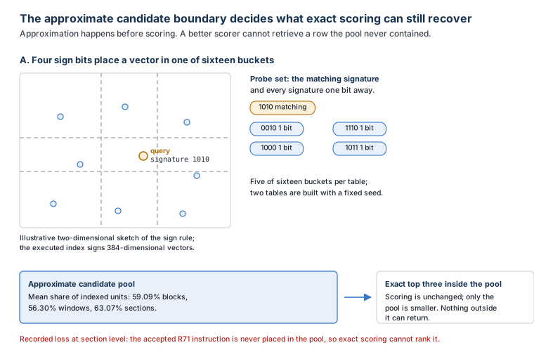
The planes, bucket assignments, parameters and unit manifests are frozen, so the same inputs rebuild the same adapter. This is a deliberately small locality-sensitive hashing (LSH) example. It does not implement HNSW, benchmark vector databases or represent ANN methods in general.
Ask two different recall questions
We need two measures because reproducing a neighbour list is not the same as retrieving useful evidence. Approximation recall at three asks what fraction of the exact top-three reference identities also appears in the approximate top three, even when none is relevant. Bundle coverage at three asks whether the selected units contain all required source evidence defined in Chapter 06. Approximation recall is averaged over every query, including no-answer cases; bundle-coverage denominators include only answerable needs.
Our identity-based measure is stricter than the distance-threshold recall used in ANN-Benchmarks, which can accept a different point tied at the exact cutoff distance. We require the particular identities selected by our declared tie order. Two equally close vectors may therefore count as interchangeable under a distance-based benchmark but not here: their source-qualified evidence references are different.
The fixed LSH comparison gives the following results on Chapter 06’s reworded-query slice. This slice reuses the development evidence needs; it is not an independent test on new evidence.
| Scheme | Mean approximation recall at 3 | Exact bundle coverage at 3 | LSH bundle coverage at 3 |
|---|---|---|---|
| Blocks | 0.7500 | 4/7 | 3/7 |
| Windows | 0.8333 | 3/7 | 2/7 |
| Sections | 0.7500 | 6/7 | 5/7 |
The section-level loss is the R71 request: exact search ranks the accepted twenty-second instruction first, but LSH never puts it into the candidate pool. The window scheme loses the relevant final window for the reworded selector-tail query. Under blocks, the maintenance command drops out while its scope remains. These are different examples of the same boundary failure: evidence can be present in the indexed collection yet absent from the pool that the final scorer sees. The frozen traces identify the lost source spans.
Approximation can produce a favourable outcome by accident. On the development paraphrase with windows, LSH excludes higher-scoring but irrelevant neighbours; the accepted cache command then enters the selected top three. Exact search fails the bundle criterion while LSH succeeds. The index has not learned which passage is relevant. It has merely changed the candidate set, and this one fortunate exclusion is not a reason to tune parameters against the reworded-query results.
Inspect either case without rerunning the model:
python -B experiments/part2-semantic/run.py --query s-h07
python -B experiments/part2-semantic/run.py --query s-d04
Measure costs under the actual implementation
These timings cover cached-vector search inside one local Python process. For each query and method, one warm-up is excluded and twenty repetitions are timed. The reported figure is the median of the per-query medians across all eighteen queries. It excludes encoding, model loading, network transfer and current-policy projection. It therefore measures a narrow backend operation, not end-to-end retrieval latency.
The candidate-pool audit shows how much work this adapter leaves for exact reranking. Its mean pool contains 59.09% of block units, 56.30% of window units and 63.07% of section units. Each percentage is the average, across all eighteen queries including no-answer cases, of ann_pool_size divided by that scheme’s unit count. These are fairly broad candidate pools, not aggressive pruning. The timings and losses of this small LSH implementation cannot establish production ANN performance or predict HNSW behaviour.
| Scheme | Exact query ms | LSH query ms | Exact construction ms | Additional LSH construction ms |
|---|---|---|---|---|
| Blocks | 0.846 | 0.744 | 1.883 | 5.396 |
| Windows | 1.684 | 1.230 | 3.824 | 9.893 |
| Sections | 0.458 | 0.518 | 0.948 | 3.067 |
The construction figures include record copying and vector normalisation. The additional LSH construction column also includes generating hyperplanes and assigning buckets; it is incremental to building the dense index, which LSH still requires. Reading that column as the entire system’s index-build time would understate the work.
In this local run, LSH is modestly faster for block and window queries but slower for sections, while losing judged bundle coverage in all three schemes. The collections are tiny, scoring uses Python arithmetic and ranking copies records. These measurements show a trade-off in this implementation; they do not establish statistical confidence, concurrent throughput, tail latency or a production speedup.
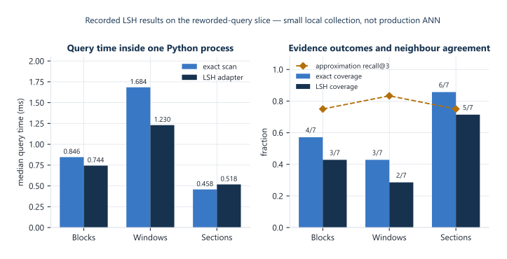
The retained storage figures also describe different things:
| Scheme | Float32 vector payload bytes | Additional LSH canonical-JSON bytes |
|---|---|---|
| Blocks | 50,688 | 89,408 |
| Windows | 102,912 | 90,287 |
| Sections | 26,112 | 88,894 |
The vector column counts rows × 384 dimensions × four bytes: the nominal float32 payload. The running Python index holds normalised Python values rather than a packed float32 matrix. The LSH column is additional canonical JSON for planes and buckets, not compressed binary index storage. Neither column measures resident or peak memory, which remains not measured. A packed implementation would need separate measurements.
Choose against losses you can inspect
HNSW makes a different approximation trade-off. Instead of assigning vectors to hash buckets, it navigates a layered proximity graph: upper layers guide the search towards a promising region, while lower-layer exploration gathers neighbours. Its graph connectivity, construction procedure and search breadth carry costs that cannot be inferred from the number of LSH tables or probes. Comparing HNSW with exact search would require its own index-build, memory, latency and neighbour-quality measurements. None was performed here.
The exact scan is a diagnostic reference, not a blanket recommendation against ANN. Index choice depends on collection scale, update frequency, current-policy requirements and how much loss of required evidence is tolerable. Probing more LSH buckets might recover some missing candidates, but it would change both work and results and require a separately declared experiment. We did not tune the adapter after observing these misses.
Both exact and approximate search operate on a particular indexed view. Even perfect agreement with exact neighbours says nothing about whether an old access decision remains valid. Filters, Scope, and Freshness takes up that next failure: an index may faithfully retrieve a passage that the current request must no longer receive.
References and further reading
Background and extensions for this chapter:
- Malkov and Yashunin (2018). Efficient and robust approximate nearest neighbor search using Hierarchical Navigable Small World graphs. arXiv preprint, v4. Provides a graph-based ANN design to compare with exact nearest neighbours.
- Johnson, Douze and Jégou (2017). Billion-scale similarity search with GPUs. arXiv preprint, v1. Extends index choice to exact, approximate and compressed search on GPUs.
- Aumüller, Bernhardsson and Faithfull (2018). ANN-Benchmarks: A Benchmarking Tool for Approximate Nearest Neighbor Algorithms. arXiv preprint, v1. Supports comparing neighbour quality with speed under a common benchmarking interface.
Related chapters
- From Similarity to Search. Compares exact and approximate vector search as separate execution choices.