Cellular Automata: Custom Rules
Introduction
This post will discuss Custom Rules for Cellular Automata
Designing Custom Rules
Custom rules allow you to tailor cellular automata to specific problems or behaviors. Unlike fixed rule sets (e.g., Rule 30), custom rules let you modify state transitions based on unique logic.
Writing Python Functions for Rule Sets
Custom rules can be implemented as Python functions that take the current cell state and its neighbors as inputs.
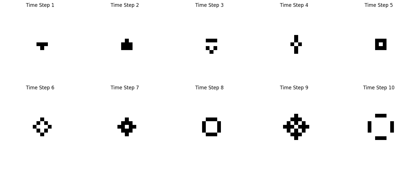
Custom Rule in 2D
This will generate a blinking effect.
import numpy as np
import matplotlib.pyplot as plt
from matplotlib import animation
from IPython.display import HTML

def custom_rule(grid, x, y):
    """Custom rule for state transition."""
    neighbors = grid[x-1:x+2, y-1:y+2].sum() - grid[x, y]
    if grid[x, y] == 1:  # Alive
        return 1 if neighbors in [2, 3] else 0
    else:  # Dead
        return 1 if neighbors == 3 else 0

def apply_custom_rule(grid, steps):
    """Applies the custom rule over multiple steps."""
    rows, cols = grid.shape
    grids = [grid]  # Store initial grid
    for _ in range(steps):
        new_grid = grid.copy()
        for x in range(1, rows-1):
            for y in range(1, cols-1):
                new_grid[x, y] = custom_rule(grid, x, y)
        grid = new_grid
        grids.append(grid)  # Store grid at each step
    return grids

# Initial grid
grid = np.zeros((20, 20), dtype=int)
grid[9, 9] = grid[9, 10] = grid[9, 11] = grid[10, 10] = 1  # Glider-like structure

# Number of steps for the simulation
num_steps = 10

# Get the grid states for each step
grids = apply_custom_rule(grid, num_steps)

# Set up the plot
fig, ax = plt.subplots(figsize=(12, 6))

# Function to update the plot for each frame
def animate(i):
    ax.clear()
    ax.imshow(grids[i], cmap='binary', interpolation='none')  # Display the grid
    ax.set_title(f'Time Step {i+1}')
    ax.set_xlabel('Position on Grid')
    ax.set_yticks([])  # Remove y-ticks for cleaner visualization

# Create the animation
anim = animation.FuncAnimation(fig, animate, frames=num_steps, interval=500)  # 500ms interval between frames

# Display the animation inline in the notebook
plt.close()  # Close the plot to avoid duplicate display
HTML(anim.to_jshtml())
Modelling the spread of Wild fire using cellular automata
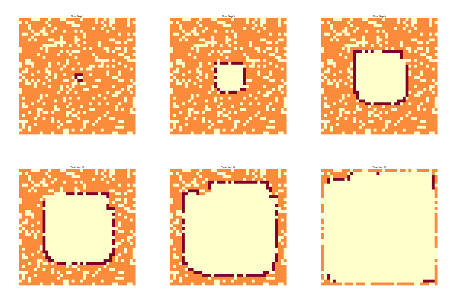
In this example we are going to model how a fire would spread in dry bush.
import numpy as np
import matplotlib.pyplot as plt
from matplotlib import animation
from IPython.display import HTML

def custom_fire_rule(grid, x, y):
    """Custom rule for fire spread in a forest."""
    if grid[x, y] == 2:  # Burning tree
        return 0  # It burns out and becomes empty
    elif grid[x, y] == 1:  # Tree
        # A tree catches fire if one of its neighbors is burning
        neighbors = grid[x-1:x+2, y-1:y+2]  # 3x3 grid around the cell
        if np.any(neighbors == 2):  # Check if any neighboring cell is burning
            return 2  # The tree catches fire
    return grid[x, y]  # Otherwise, the state stays the same (empty or tree)

def apply_fire_rule(grid, steps):
    """Applies the custom fire spread rule over multiple steps."""
    rows, cols = grid.shape
    for _ in range(steps):
        new_grid = grid.copy()
        for x in range(1, rows-1):
            for y in range(1, cols-1):
                new_grid[x, y] = custom_fire_rule(grid, x, y)
        grid = new_grid
        yield grid

# Initialize a larger forest grid (40x40)
forest = np.zeros((40, 40), dtype=int)

# Increase the probability of trees to 0.8 (80% of cells will be trees)
np.random.seed(42)  # For reproducibility
forest = np.random.choice([0, 1], size=(40, 40), p=[0.2, 0.8])  # 80% trees, 20% empty cells

# Set an initial fire at the center
forest[20, 20] = 2  # Starting fire at the center of the forest

# Number of steps for the simulation
num_steps = 20

# Get the state of the forest over multiple time steps
forest_states = list(apply_fire_rule(forest, steps=num_steps))

# Set up the subplots for displaying the simulation steps
fig, ax = plt.subplots(figsize=(12, 12))  # Adjusted size for the larger grid

def animate_fire(i):
    """Animate the forest fire spread."""
    ax.clear()  # Clear the axis for the next step
    ax.imshow(forest_states[i], cmap='YlOrRd', interpolation='none')  # Display the forest grid
    ax.set_title(f'Time Step {i+1}')
    ax.axis('off')  # Turn off the axis

# Create the animation
anim = animation.FuncAnimation(fig, animate_fire, frames=len(forest_states), interval=500)

# Display the animation in Jupyter Notebook
plt.close()  # Close the plot to prevent duplicate display
HTML(anim.to_jshtml())
Exploring Edge Cases and Behaviors
When designing custom rules:
- Test for edge cases such as boundary conditions (e.g., wrap-around grids).
- Evaluate stability and emergent properties, such as oscillations or chaos.
- Add debug visualizations to verify that transitions behave as expected.
Debugging Edge Cases
If you can generate gifs like in this post it will help, otherwise add logging or signals.
# Debugging the behavior of edges
print(f"Initial State:\n{grid}")
for i, g in enumerate(apply_custom_rule(grid, 2)):
    print(f"After Step {i + 1}:\n{g}")
Multi-Dimensional Grids
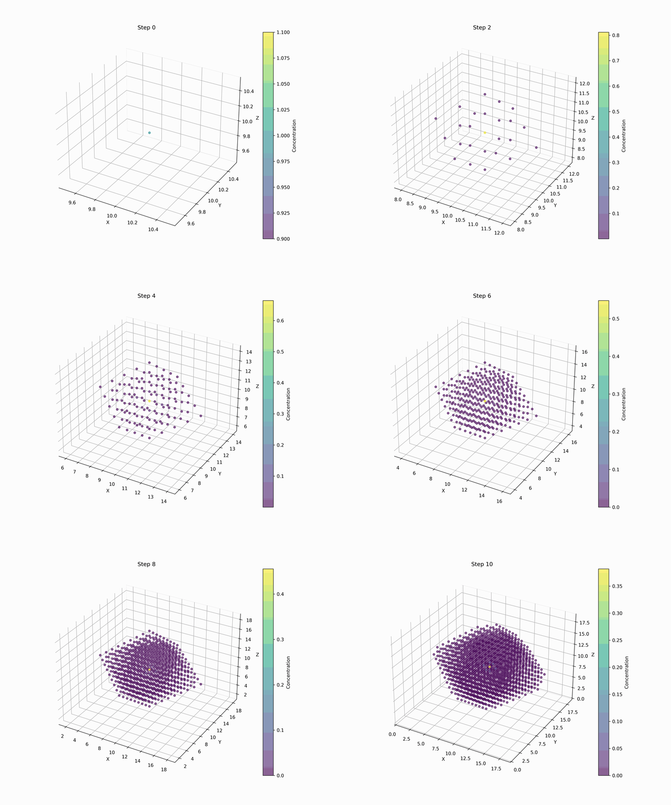
Extending cellular automata to three or more dimensions allows the simulation of volumetric phenomena, such as fluid dynamics, diffusion, and even 3D patterns in generative art.
3D Cellular Automaton
Here we are modelling a diffusion process.
import numpy as np
import matplotlib.pyplot as plt
from mpl_toolkits.mplot3d import Axes3D
from matplotlib import animation
from IPython.display import HTML

def initialize_grid_3d(size, concentration=1.0):
    """
    Initializes a 3D grid with a localized concentration in the center.
    """
    grid = np.zeros((size, size, size))
    center = size // 2
    grid[center, center, center] = concentration
    return grid

def diffusion_rule(grid, diffusion_rate=0.1):
    """
    Applies a simple diffusion rule to the 3D grid.
    Each cell exchanges a fraction of its concentration with its neighbors.
    """
    new_grid = grid.copy()
    size = grid.shape[0]

    for x in range(1, size - 1):
        for y in range(1, size - 1):
            for z in range(1, size - 1):
                # Compute the average concentration of neighbors
                neighbors = (
                    grid[x-1, y, z] + grid[x+1, y, z] +
                    grid[x, y-1, z] + grid[x, y+1, z] +
                    grid[x, y, z-1] + grid[x, y, z+1]
                ) / 6.0

                # Update the cell concentration
                new_grid[x, y, z] += diffusion_rate * (neighbors - grid[x, y, z])

    return new_grid

def simulate_diffusion(grid, steps, diffusion_rate=0.1):
    """
    Simulates the diffusion process over a number of time steps.
    """
    states = [grid]
    for _ in range(steps):
        grid = diffusion_rule(grid, diffusion_rate)
        states.append(grid)
    return states

def visualize_diffusion_step(grid, step, save_path=None):
    """
    Visualizes a single step of the 3D diffusion grid as a scatter plot.
    """
    fig = plt.figure(figsize=(10, 8))
    ax = fig.add_subplot(111, projection='3d')

    size = grid.shape[0]
    x, y, z = np.meshgrid(np.arange(size), np.arange(size), np.arange(size), indexing='ij')
    concentrations = grid.flatten()

    # Use only non-zero points for visualization
    nonzero_indices = concentrations > 0
    sc = ax.scatter(x.flatten()[nonzero_indices],
                    y.flatten()[nonzero_indices],
                    z.flatten()[nonzero_indices],
                    c=concentrations[nonzero_indices],
                    cmap='viridis', alpha=0.6)

    ax.set_title(f"Step {step}")
    ax.set_xlabel("X")
    ax.set_ylabel("Y")
    ax.set_zlabel("Z")
    plt.colorbar(sc, ax=ax, label="Concentration")

    if save_path:
        plt.savefig(save_path, dpi=300)
    plt.close(fig)

# Parameters
grid_size = 20
time_steps = 10
diffusion_rate = 0.1

# Initialize grid and simulate
initial_grid = initialize_grid_3d(size=grid_size, concentration=1.0)
diffusion_states = simulate_diffusion(initial_grid, steps=time_steps, diffusion_rate=diffusion_rate)

# Save each step as an image for GIF creation
image_filenames = []
for step, state in enumerate(diffusion_states):
    filename = f"diffusion_step_{step}.png"
    visualize_diffusion_step(state, step, save_path=filename)
    image_filenames.append(filename)

# Create GIF from saved images
def create_gif(image_filenames, output_filename="diffusion_simulation.gif", fps=2):
    """
    Creates an animated GIF from a list of image filenames.
    """
    from PIL import Image
    images = [Image.open(filename) for filename in image_filenames]
    images[0].save(output_filename, save_all=True, append_images=images[1:], duration=1000 // fps, loop=0)

GIF_FILENAME = "diffusion_simulation.gif"

create_gif(image_filenames, output_filename=GIF_FILENAME, fps=2)

# Display the GIF in Jupyter Notebook
from IPython.display import Image
Image(filename=GIF_FILENAME)
Applications in Volumetric Simulations
- Diffusion: Simulating the spread of particles in 3D space.
- Physics: Modeling structures like crystals or magnetic domains.
- Art: Generating 3D patterns for rendering or 3D printing.
Visualization Tip:
Use libraries like matplotlib for 3D plots or mayavi for advanced visualization.
Stochastic Cellular Automata
Stochastic automata introduce randomness into rule evaluation, making them ideal for simulating probabilistic systems like diffusion, noise, and random growth.
Extending the forest fire example
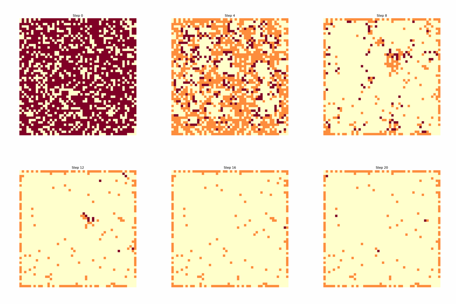
Forest fire model implemented using stochastic CA, where trees catch fire with a probability depending on their neighbors.
import numpy as np
import matplotlib.pyplot as plt
from matplotlib import animation
from IPython.display import HTML

def initialize_forest(size, tree_prob=0.6):
    """
    Initializes the forest grid with trees and empty spaces.
    `tree_prob` defines the probability of a cell being a tree.
    """
    return np.random.choice([0, 1], size=(size, size), p=[1 - tree_prob, tree_prob])

def stochastic_fire_rule(grid, prob_ignite=0.2, prob_spread=0.6):
    """
    Applies the stochastic fire spread rule to the grid.
    States:
      0 - Empty
      1 - Tree
      2 - Burning
    """
    new_grid = grid.copy()
    size = grid.shape[0]
    for x in range(1, size - 1):
        for y in range(1, size - 1):
            if grid[x, y] == 1:  # Tree
                # A tree ignites randomly with probability `prob_ignite`
                if np.random.rand() < prob_ignite:
                    new_grid[x, y] = 2
                # A tree catches fire if any neighbor is burning
                elif np.any(grid[x-1:x+2, y-1:y+2] == 2) and np.random.rand() < prob_spread:
                    new_grid[x, y] = 2
            elif grid[x, y] == 2:  # Burning tree
                # A burning tree becomes empty
                new_grid[x, y] = 0
    return new_grid

def simulate_fire(grid, steps, prob_ignite=0.2, prob_spread=0.6):
    """
    Simulates the stochastic forest fire over a number of steps.
    """
    states = [grid]
    for _ in range(steps):
        grid = stochastic_fire_rule(grid, prob_ignite, prob_spread)
        states.append(grid)
    return states

def visualize_fire_step(grid, step, save_path=None):
    """
    Visualizes a single step of the forest fire grid.
    """
    fig, ax = plt.subplots(figsize=(8, 8))
    cmap = plt.cm.get_cmap("YlOrRd", 3)  # Define colors for the three states
    ax.imshow(grid, cmap=cmap, interpolation="none")
    ax.set_title(f"Step {step}")
    ax.axis("off")
    if save_path:
        plt.savefig(save_path, dpi=300)
    plt.close(fig)

# Parameters
grid_size = 50
tree_prob = 0.7
time_steps = 20
prob_ignite = 0.02
prob_spread = 0.6

# Initialize the forest and simulate
forest = initialize_forest(grid_size, tree_prob=tree_prob)
forest_states = simulate_fire(forest, time_steps, prob_ignite=prob_ignite, prob_spread=prob_spread)

# Save images for visualization
image_filenames = []
for step, state in enumerate(forest_states):
    filename = f"forest_fire_step_{step}.png"
    visualize_fire_step(state, step, save_path=filename)
    image_filenames.append(filename)

# Create an animated GIF
def create_gif(image_filenames, output_filename="stochastic_forest_fire.gif", fps=2):
    """
    Creates an animated GIF from a list of image filenames.
    """
    from PIL import Image
    images = [Image.open(filename) for filename in image_filenames]
    images[0].save(output_filename, save_all=True, append_images=images[1:], duration=1000 // fps, loop=0)

create_gif(image_filenames, output_filename="stochastic_forest_fire.gif", fps=2)

# Display the GIF
from IPython.display import Image
Image(filename="stochastic_forest_fire.gif")
This generates the following image:
How the Stochastic Model Works
States:
0: Empty 1: Tree 2: Burning Rules:
Trees catch fire probabilistically, either spontaneously (ignition probability) or if neighbors are burning (spread probability). Burning trees turn into empty cells in the next step. Visualization:
The model shows how fires spread probabilistically through a forest grid. The randomness ensures varied outcomes for each simulation.
Simulating Noise and Probabilistic Systems
Stochastic cellular automata can be used for:
- Noise Generation: Simulate random patterns for texture or testing.
- Biological Models: Capture probabilistic behaviors like mutation or infection spread.
- Monte Carlo Simulations: Model uncertainty and randomness in physical systems.
Further References
- Stochastic Cellular Automata:
- 3D Visualization in Python:
- Multi-State Automata:
- Wolfram’s N-State Cellular Automata
Code Examples
Check out the ca notebooks for the code used in this post and additional examples.
Summary
We explored ways to customize cellular automata, including defining custom rules, extending to multi-dimensional grids, and introducing stochastic elements. These techniques empower programmers to simulate increasingly realistic and complex systems.
