Build a Forest Fire Simulation
Cellular Automata From First Principles 09: Build a Forest Fire Simulation
A forest fire is almost an ideal cellular-automaton exercise.
The visible states are obvious:
0 = empty
1 = tree
2 = burning
The interactions are local.
And small changes in fuel density or ignition assumptions can produce very different global outcomes.
This is not intended as a high-fidelity wildfire model.
It is a deliberately simplified spread model designed to isolate one mechanism:
How does local fuel connectivity determine whether fire propagates through a landscape?
Initialize the forest
import numpy as np

EMPTY = 0
TREE = 1
FIRE = 2


def make_forest(
    rows=150,
    cols=200,
    tree_density=0.65,
    seed=42,
):
    rng = np.random.default_rng(seed)

    grid = np.zeros(
        (rows, cols),
        dtype=np.uint8,
    )

    grid[
        rng.random((rows, cols)) < tree_density
    ] = TREE

    return grid
Ignite one cell:
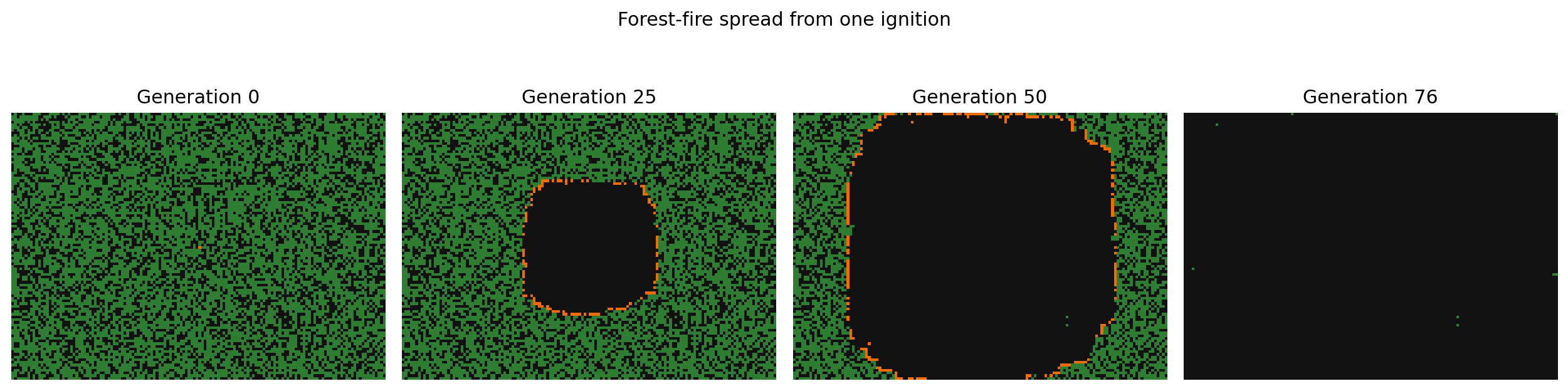
forest = make_forest()

forest[
    forest.shape[0] // 2,
    forest.shape[1] // 2,
] = FIRE
Now tree_density becomes an experimental parameter.
At low density, burning regions may encounter gaps.
At high density, the tree network may become connected enough for fire to travel much farther.
Detect burning neighbors without wraparound
For a literal forest map, the left edge should not normally touch the right edge.
That means periodic np.roll boundaries would create a modeling artifact.
A useful helper is a fixed-edge shift:
def shift_fixed(a, dy, dx):
    out = np.zeros_like(a)

    src_y0 = max(0, -dy)
    src_y1 = a.shape[0] - max(0, dy)
    src_x0 = max(0, -dx)
    src_x1 = a.shape[1] - max(0, dx)

    dst_y0 = max(0, dy)
    dst_y1 = a.shape[0] - max(0, -dy)
    dst_x0 = max(0, dx)
    dst_x1 = a.shape[1] - max(0, -dx)

    out[
        dst_y0:dst_y1,
        dst_x0:dst_x1,
    ] = a[
        src_y0:src_y1,
        src_x0:src_x1,
    ]

    return out
Then:
def burning_neighbor_mask(grid):
    burning = grid == FIRE
    near_fire = np.zeros_like(
        burning,
        dtype=bool,
    )

    for dy in (-1, 0, 1):
        for dx in (-1, 0, 1):
            if dy == 0 and dx == 0:
                continue

            near_fire |= shift_fixed(
                burning,
                dy,
                dx,
            )

    return near_fire
Boundary behavior is part of the model, so it should be visible in the implementation.
Write one synchronous update
def forest_step(
    grid,
    rng,
    lightning_probability=0.0,
):
    next_grid = grid.copy()

    burning = grid == FIRE
    trees = grid == TREE
    near_fire = burning_neighbor_mask(grid)

    next_grid[burning] = EMPTY

    ignite_from_neighbor = trees & near_fire

    lightning = (
        trees
        & (
            rng.random(grid.shape)
            < lightning_probability
        )
    )

    next_grid[
        ignite_from_neighbor | lightning
    ] = FIRE

    return next_grid
Each transition remains readable.
burning -> empty

tree + burning neighbor -> burning

tree + lightning event -> burning
That readability matters more than compressing the entire rule into one expression.
Run until the fire dies out
def run_fire(
    initial,
    steps=250,
    seed=123,
    lightning_probability=0.0,
):
    rng = np.random.default_rng(seed)
    grid = initial.copy()
    history = []

    for _ in range(steps):
        history.append(grid.copy())

        if (
            not np.any(grid == FIRE)
            and lightning_probability == 0
        ):
            break

        grid = forest_step(
            grid,
            rng,
            lightning_probability,
        )

    return history
With spontaneous ignition disabled:
no burning cells
      ->
no future burning cells
That is a useful termination invariant.
Measure the state populations
The animation tells us where the fire moved.
Population curves tell us what the process did overall.
def state_counts(grid):
    return {
        "empty": int(
            np.count_nonzero(grid == EMPTY)
        ),
        "trees": int(
            np.count_nonzero(grid == TREE)
        ),
        "burning": int(
            np.count_nonzero(grid == FIRE)
        ),
    }
Collect that every generation.
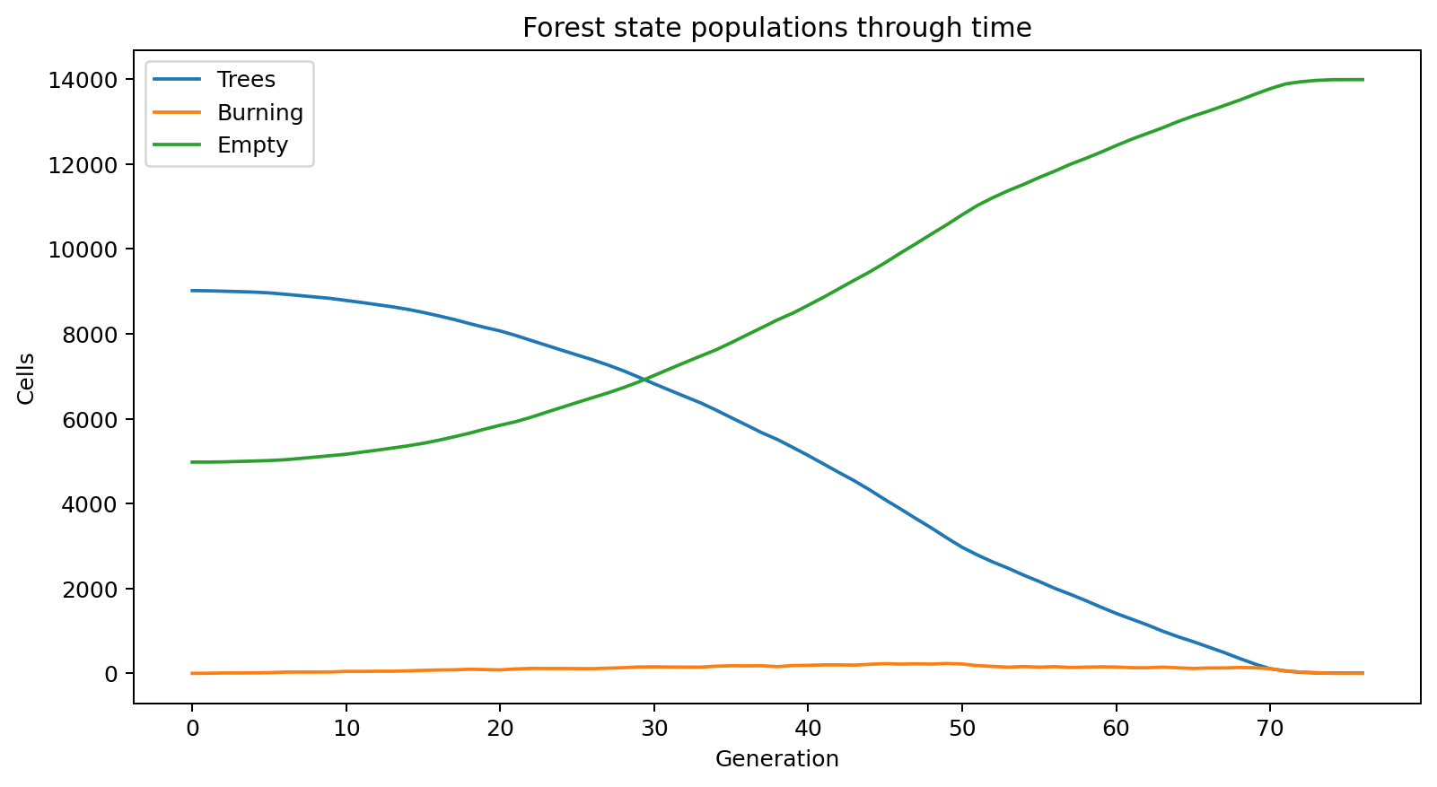
The burning population rises while connected fuel is available, then collapses as the local front runs out of reachable trees.
Measure burn fraction
def fire_summary(initial, final):
    initial_trees = np.count_nonzero(
        initial == TREE
    )

    surviving_trees = np.count_nonzero(
        final == TREE
    )

    burned = initial_trees - surviving_trees

    return {
        "initial_trees": int(initial_trees),
        "surviving_trees": int(
            surviving_trees
        ),
        "burned": int(burned),
        "burn_fraction": (
            burned / initial_trees
            if initial_trees
            else 0.0
        ),
    }
Now sweep density across many seeds.
That experiment is more informative than selecting one dramatic animation.
We can ask:
At density d,
what is the distribution of burn fractions?
That question separates a stochastic realization from a model-level claim.
Add direction only when the mechanism demands it
The current model treats all neighboring directions equally.
A wind-biased model would not.
Conceptually:
burning neighbor west of tree
    -> higher ignition probability

burning neighbor east of tree
    -> lower ignition probability
That changes the neighborhood from an unordered collection into a directional one.
The general lesson is:
An anisotropic world requires an anisotropic local rule.
Do not add wind as a cosmetic animation effect. Put it into the transition probabilities.
Add regrowth to create a persistent system
If empty cells can regrow trees and trees can ignite spontaneously, the world no longer terminates.
A slow regrowth process can compete with a fast burning process:
slow:
trees accumulate
      ↓
fuel network forms

fast:
ignition occurs
      ↓
fire consumes connected fuel
The interaction between timescales can generate long-running global dynamics.
One idea to keep
This chapter is not valuable because it looks like a fire.
It is valuable because we can state exactly what the model contains:
space
state
neighborhood
boundary condition
spread rule
random process
initial fuel density
and then ask how changing one ingredient alters the outcome distribution.
In the next chapter we will use the same local viewpoint for a conserved moving quantity: cars on a one-dimensional road.
