Simulate Traffic with Rule 184
Cellular Automata From First Principles 10: Simulate Traffic with Rule 184
Rule 184 is a beautiful example of moving from an abstract rule table to a model with a concrete interpretation.
Use a one-dimensional ring road:
1 = car
0 = empty road
A car moves one cell to the right when the destination is empty.
That is enough to produce free flow, queues and a macroscopic density-flow relationship.
Write the traffic mechanism directly
import numpy as np


def traffic_step(road):
    cars = road == 1

    empty_ahead = (
        np.roll(road, -1) == 0
    )

    moving = cars & empty_ahead

    next_road = road.copy()

    next_road[moving] = 0
    next_road[
        np.roll(moving, 1)
    ] = 1

    return next_road
The road is periodic, so the final road cell connects back to the first.
For this model that is deliberate:
closed ring road
not an implementation accident.
Conservation gives us a strong invariant
Cars do not appear or disappear:
road = np.array(
    [1, 0, 1, 1, 0, 0, 1],
    dtype=np.uint8,
)

next_road = traffic_step(road)

assert road.sum() == next_road.sum()
That invariant is stronger than testing only a few expected cells.
It expresses something the model must preserve under every valid update.
Initialize by density
def make_road(
    length=240,
    density=0.35,
    seed=42,
):
    rng = np.random.default_rng(seed)

    return (
        rng.random(length) < density
    ).astype(np.uint8)
Run it:
road = make_road(density=0.62)

history = []

for _ in range(180):
    history.append(road.copy())
    road = traffic_step(road)

history = np.array(history)
Because rows represent time and columns represent road position, the result is another spacetime diagram.
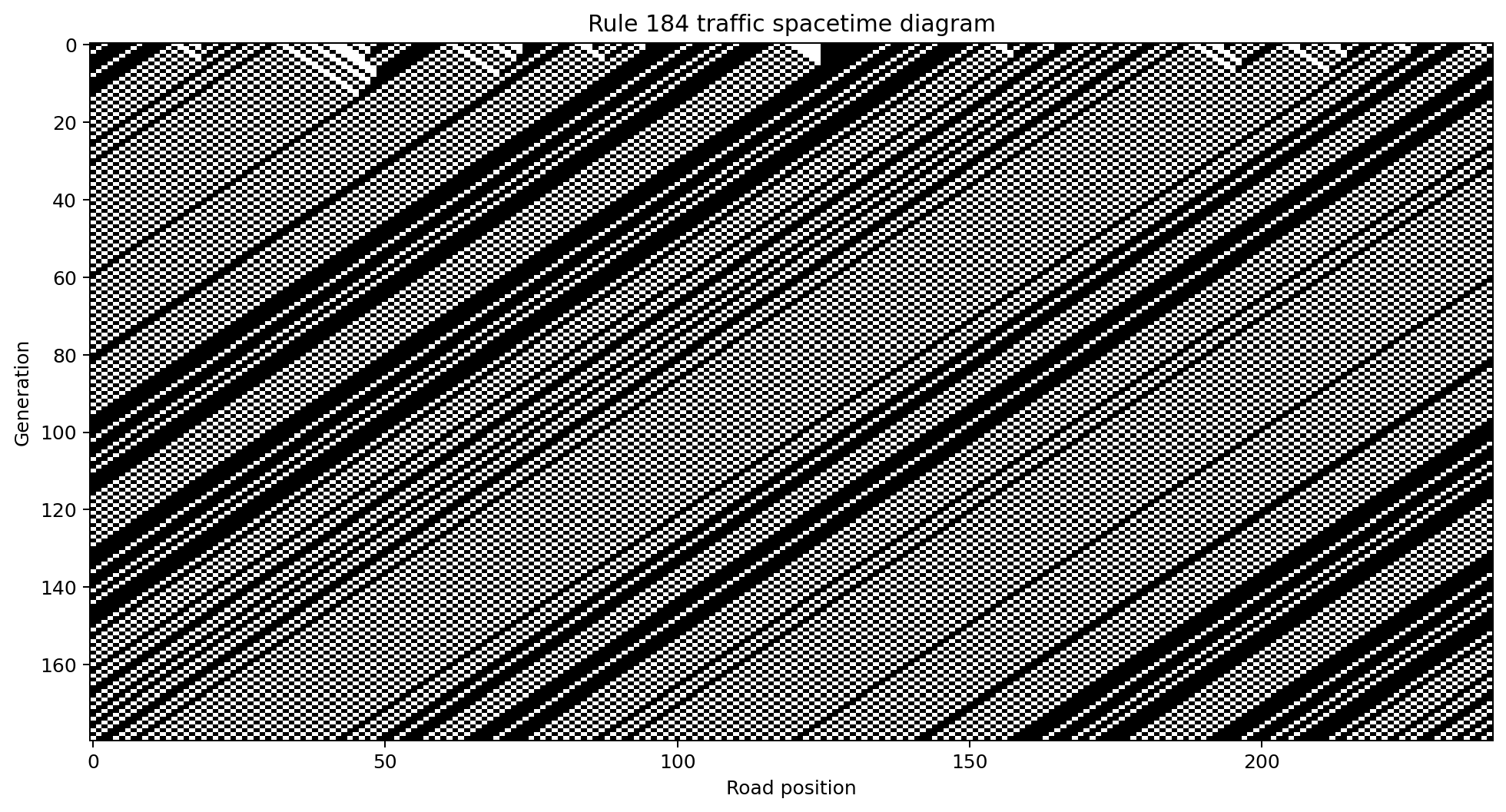
Diagonal traces show cars advancing.
Dense structures reveal blocked movement.
One local exclusion rule is enough to create collective congestion.
Measure movement, not only occupancy
Density tells us how much of the road is occupied.
Flow tells us how much movement occurs.
def traffic_step_with_flow(road):
    cars = road == 1

    empty_ahead = (
        np.roll(road, -1) == 0
    )

    moving = cars & empty_ahead

    next_road = road.copy()
    next_road[moving] = 0
    next_road[
        np.roll(moving, 1)
    ] = 1

    return next_road, int(moving.sum())
Normalize movement by road length:
flow_per_cell = moving_cars / len(road)
Now sweep density after allowing a warm-up period.
def average_flow(
    density,
    steps=700,
    warmup=200,
    length=600,
    seed=1,
):
    road = make_road(
        length,
        density,
        seed,
    )

    values = []

    for t in range(steps):
        road, moving = (
            traffic_step_with_flow(road)
        )

        if t >= warmup:
            values.append(
                moving / length
            )

    return float(np.mean(values))
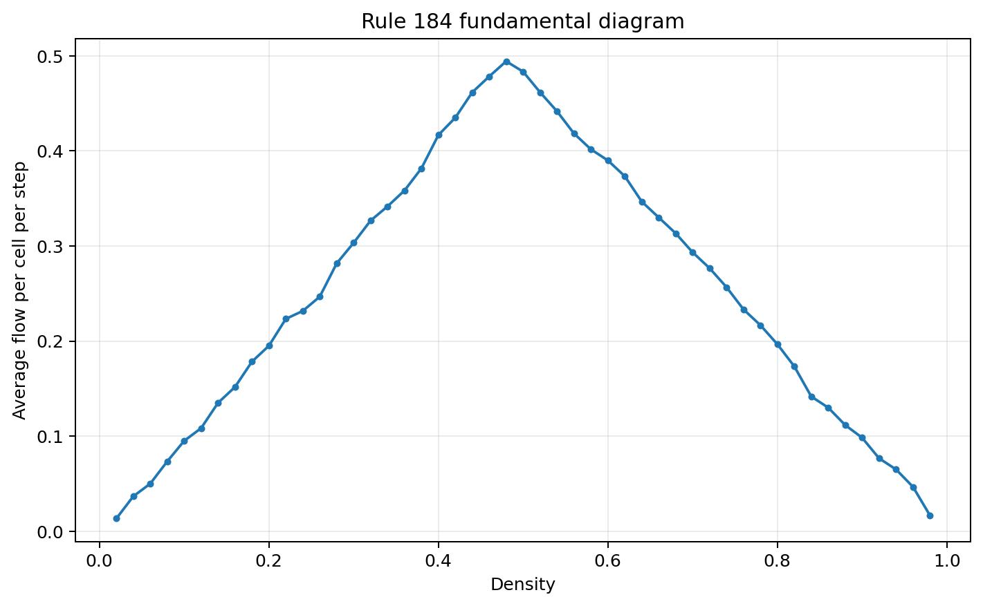
For deterministic Rule 184 on a ring, the characteristic shape is easy to interpret:
low density:
few cars exist
-> low total flow

intermediate density:
many cars can move
-> high flow

high density:
empty destinations are scarce
-> flow falls
The macroscopic relationship is not coded directly.
It emerges from local occupancy constraints.
A traffic jam is an observer-level object
No cell contains:
JAM = True
No car computes queue length.
Each car only needs to know:
am I here?
is the cell ahead empty?
Yet we can observe a persistent region of blocked vehicles and call it a traffic jam.
This is the same ontological split we saw with gliders:
implementation:
bits + local rules

observer:
cars + queues + flow
Add stochastic slowing
Real drivers do not always move whenever space is available.
A hesitation probability adds another mechanism:
def stochastic_traffic_step(
    road,
    rng,
    slow_probability=0.1,
):
    cars = road == 1

    empty_ahead = (
        np.roll(road, -1) == 0
    )

    willing = (
        rng.random(len(road))
        >= slow_probability
    )

    moving = (
        cars
        & empty_ahead
        & willing
    )

    next_road = road.copy()
    next_road[moving] = 0
    next_road[
        np.roll(moving, 1)
    ] = 1

    return next_road
Now two sources can reduce flow:
physical blocking
random hesitation
Those should be measured separately.
Rule 184 is one traffic model, not traffic itself
The model assumes:
one lane
one cell per vehicle
maximum speed one cell per step
no overtaking
closed ring road
synchronous updates
Those assumptions are useful because they isolate the mechanism.
A richer model can add velocity, braking, lane changes or open boundaries.
But the discipline stays the same:
Start from the smallest local information needed to express the mechanism you care about.
One idea to keep
Rule 184 turns a microscopic rule into a macroscopic observable.
That gives us a useful experimental pattern:
local update
    ↓
trajectory
    ↓
observable
    ↓
parameter sweep
    ↓
emergent relationship
In the next chapter we will apply that pattern to a continuous quantity and show how local exchange creates diffusion.
