Cellular Automata From First Principles 11: Diffusion as Local Exchange

Until now most cells have stored discrete state:

0 / 1
empty / tree / fire
road / car

Now let each cell store a continuous quantity.

For diffusion:

state[y, x] = concentration

The local transition is no longer birth, death or movement.

It is local exchange.

Start with a pulse

import numpy as np

size = 121

grid = np.zeros(
    (size, size),
    dtype=np.float64,
)

grid[
    size // 2,
    size // 2,
] = 1.0

At the beginning one cell contains all the concentration.

Repeated local exchange should spread that quantity outward.

The discrete Laplacian

A four-neighbor periodic Laplacian is:

def laplacian(grid):
    return (
        np.roll(grid, 1, axis=0)
        + np.roll(grid, -1, axis=0)
        + np.roll(grid, 1, axis=1)
        + np.roll(grid, -1, axis=1)
        - 4 * grid
    )

Interpret it locally.

If a cell is higher than its neighbors, the Laplacian tends to be negative.

If it is lower than its neighbors, the Laplacian tends to be positive.

So it tells us which way local differences should relax.

One explicit diffusion step

def diffusion_step(
    grid,
    rate=0.15,
):
    return (
        grid
        + rate * laplacian(grid)
    )

Run it:

for _ in range(120):
    grid = diffusion_step(grid)

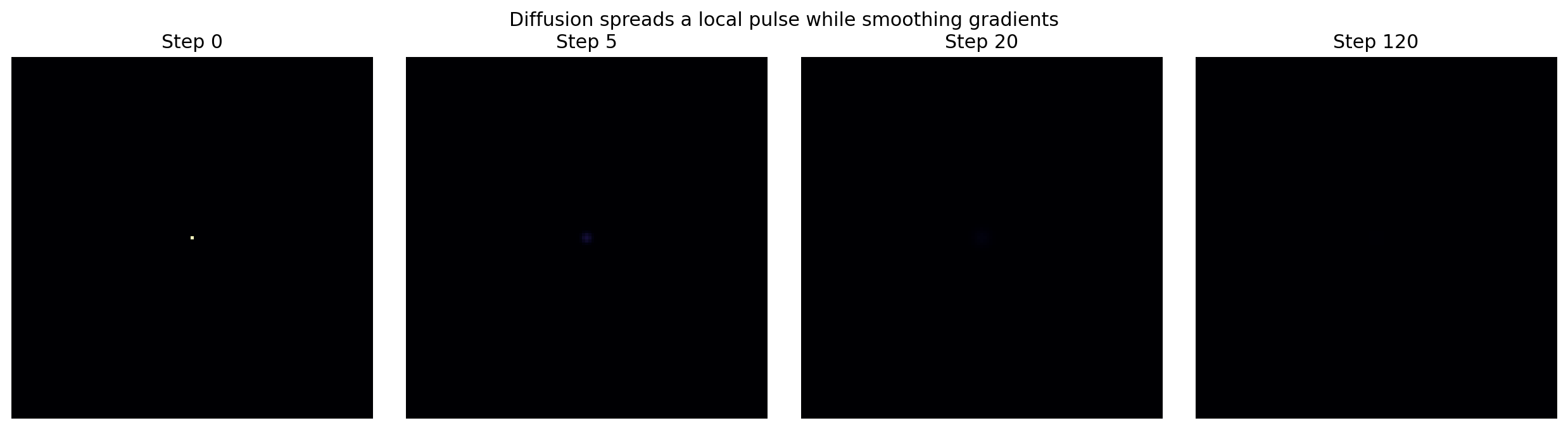
The pulse spreads without any cell knowing where the source was.

There is no global smoothing operator examining the whole map.

Every update is assembled from nearest-neighbor differences.

Conservation is the first thing to test

With periodic boundaries, the Laplacian contributions sum to zero.

So this discrete update should conserve total concentration up to floating-point error.

initial_total = grid.sum()

for _ in range(50):
    grid = diffusion_step(grid)

final_total = grid.sum()

assert np.isclose(
    initial_total,
    final_total,
)

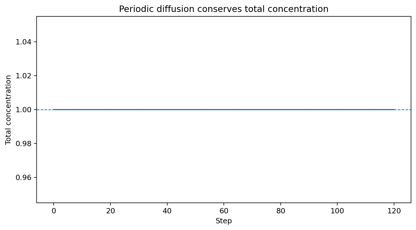
This is one reason invariants are so valuable.

A heatmap can look plausible while leaking or inventing material.

A conservation check can expose that immediately.

Why the local rule smooths differences

Consider a one-dimensional slice:

0.0  0.0  1.0  0.0  0.0

At the centre:

neighbors lower
-> negative Laplacian
-> concentration falls

At adjacent cells:

one neighbor much higher
-> positive Laplacian
-> concentration rises

Repeated updates reduce local gradients.

That is the mechanism.

Numerical stability is part of the model implementation

Try an excessively large rate:

grid = diffusion_step(
    grid,
    rate=1.0,
)

The update can oscillate, produce negative values or become unstable.

That teaches an important simulation lesson:

continuous equation
       !=
arbitrary discrete time step

A discrete implementation carries assumptions about spatial spacing, time step and numerical stability.

When we later build reaction-diffusion systems, those assumptions matter even more.

Measure spread directly

Instead of saying that the pulse “looks wider,” measure its second moment.

def spread_radius(grid):
    y, x = np.indices(grid.shape)
    total = grid.sum()

    cx = (x * grid).sum() / total
    cy = (y * grid).sum() / total

    r2 = (
        (x - cx) ** 2
        + (y - cy) ** 2
    )

    return np.sqrt(
        (r2 * grid).sum()
        / total
    )

Collect that through time and we get a quantitative measure of spreading.

The image answers:

Where is the concentration?

The metric answers:

How far has the distribution spread?

Both are useful.

Sources, sinks and obstacles change the geometry

A maintained source can keep a region at high concentration.

A sink can remove concentration.

Walls can prevent exchange across selected edges.

At that point geometry becomes part of the dynamics:

cell values
+
which neighbors can exchange
=
effective transport network

This is a recurring idea.

The grid is not merely storage.

Its connectivity determines possible causal interactions.

Continuous state opens a new design space

Conceptually we moved from:

state[y, x] = 0 or 1

to:

state[y, x] = concentration

Soon we will move again:

state[y, x] = [u, v]

and later:

state[y, x, channel]

The cell is becoming a local vector of interacting state.

One idea to keep

Pure diffusion removes local differences.

Left alone, it tends to erase structure.

So if we want persistent spots, stripes or moving boundaries, something must compete with that smoothing process.

In the next chapter we will add a local reaction to two diffusing fields and build a Gray-Scott reaction-diffusion system.