Generate Textures with Local Rules
Cellular Automata From First Principles 16: Generate Textures with Local Rules
Cellular automata do not need to represent a literal physical system.
They can also be used as visual machines.
The same ingredients we have used throughout the book:
local state
neighborhood perception
shared update
repetition
can generate masks, growth patterns, surface variation and animation.
The evaluation question changes.
Instead of asking:
Is this physically accurate?
we ask:
Does this local process produce useful, controllable visual structure?
That still demands more than “it looks interesting.”
Start with raw scalar noise
import numpy as np

rng = np.random.default_rng(42)

texture = rng.random(
    (160, 160)
)
Raw noise contains variation but little coherent structure.
A local process can create spatial correlation.
Smooth and sharpen locally
def neighborhood_mean(grid):
    total = np.zeros_like(grid)

    for dy in (-1, 0, 1):
        for dx in (-1, 0, 1):
            total += np.roll(
                np.roll(
                    grid,
                    dy,
                    axis=0,
                ),
                dx,
                axis=1,
            )

    return total / 9.0
Smoothing:
def smooth(
    grid,
    amount=0.20,
):
    return (
        (1 - amount) * grid
        + amount
        * neighborhood_mean(grid)
    )
Sharpening:
def sharpen(
    grid,
    amount=0.15,
):
    mean = neighborhood_mean(grid)

    return np.clip(
        grid
        + amount * (grid - mean),
        0.0,
        1.0,
    )
Now alternate the two:
for _ in range(30):
    texture = smooth(texture)
    texture = sharpen(texture)
The result is not magic.
It is competition between:
homogenization
and
contrast amplification
Convert continuous structure into a mask
mask = texture > 0.52
The mask can later be interpreted as:
corrosion
moss
cracks
damage
cloud coverage
paint wear
biome edge
The generator does not need to know the final semantic label.
Grow material from sparse seeds
growth = (
    rng.random((160, 160))
    < 0.01
).astype(np.uint8)
Count neighbors and allow growth only near existing material.
Then add a small decay probability.
Now the system contains competing creation and removal processes.
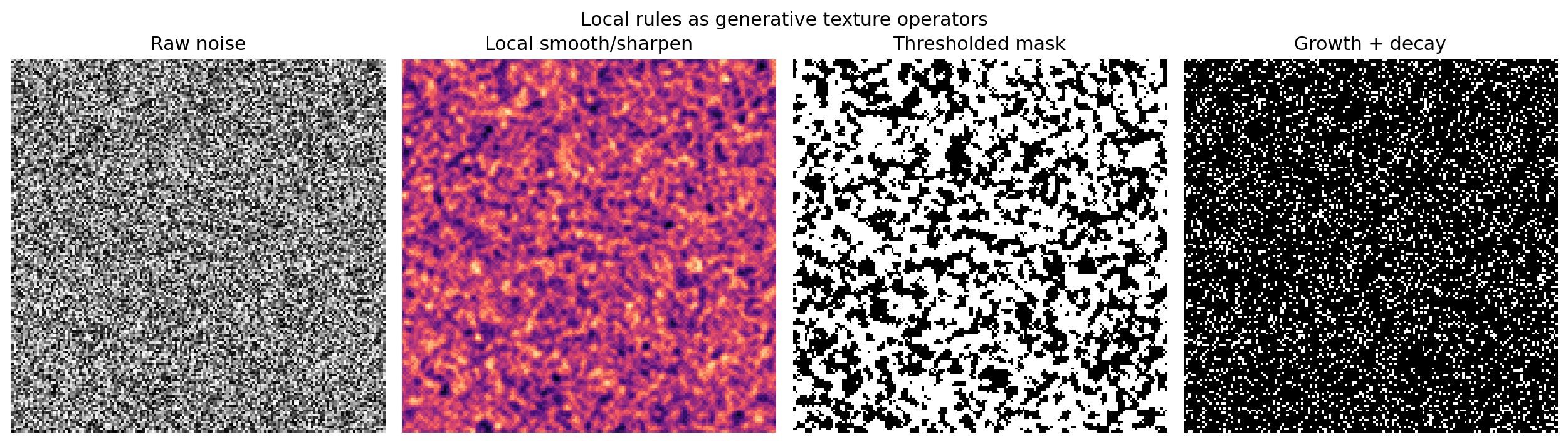
The figure compares:
raw noise
local smooth/sharpen dynamics
thresholded mask
growth + decay
That comparison is more useful than presenting four unrelated pretty images because every panel exposes a different mechanism.
Separate hidden state from rendered appearance
A richer texture system might store:
state = np.zeros(
    (160, 160, 3),
    dtype=np.float32,
)
with:
channel 0 = material
channel 1 = moisture
channel 2 = damage
The internal state can drive local updates.
A separate render function can convert it to RGB:
def render(state):
    material = state[..., 0]
    moisture = state[..., 1]
    damage = state[..., 2]

    rgb = np.stack(
        [
            material * (1 - damage),
            material * (
                1 - 0.5 * damage
            ),
            material * (
                1 - moisture
            ),
        ],
        axis=-1,
    )

    return np.clip(
        rgb,
        0.0,
        1.0,
    )
This separation becomes extremely important later.
A cell can carry information needed for local computation without every channel having a direct visual interpretation.
Animate the process, not only the result
A final frame may hide the interesting dynamics.
Store intermediate states:
frames = []

for _ in range(200):
    frames.append(
        growth.copy()
    )

    growth = growth_decay_step(
        growth,
        rng,
    )
Now the visual artifact can show:
nucleation
growth
competition
decay
reorganization
rather than only the endpoint.
For some chapters later in the book, animation will be more informative than a static PNG.
Measure useful visual properties
Aesthetic quality is partly subjective.
But we can still expose measurable properties.
Coverage
def coverage(mask):
    return float(mask.mean())
Mean local contrast
def mean_local_contrast(grid):
    return float(
        np.mean(
            np.abs(
                grid
                - neighborhood_mean(grid)
            )
        )
    )
Temporal change
def frame_change(a, b):
    return float(
        np.mean(
            np.abs(
                a.astype(float)
                - b.astype(float)
            )
        )
    )
Those metrics let us express design constraints such as:
coverage near 45%
moderate local contrast
non-zero but bounded animation rate
Search rather than hand-tune forever
candidates = []

for seed in range(100):
    rng = np.random.default_rng(seed)

    grid = (
        rng.random((128, 128))
        < 0.01
    ).astype(np.uint8)

    for _ in range(80):
        grid = growth_decay_step(
            grid,
            rng,
            grow_p=0.08,
            decay_p=0.015,
        )

    score = abs(
        coverage(grid) - 0.45
    )

    candidates.append(
        (score, seed, grid)
    )

candidates.sort(
    key=lambda x: x[0]
)
The system is programmable at two levels:
local rule
    -> produces candidate

evaluation/search
    -> chooses candidate
That is the bridge into the next part of the book.
What Part II taught us
We used one local-computation viewpoint to build:
stochastic spreading
forest fire
traffic
diffusion
reaction-diffusion
predator-prey dynamics
caves
terrain
textures
The semantics changed dramatically.
The computational skeleton did not:
local state
local perception
shared transition
repeated update
measurement
We now know how to build cellular worlds.
The next question is harder:
How do we tell which worlds are dynamically interesting?
In Part III we will measure activity, density, entropy, periodicity, attractors and sensitivity, then use those measurements to search rule space systematically.
