Calibration
Spend labels on a probability map, then measure what survives a change in distribution.
You have a queue of requests and a program that branches on a provider’s score. Confidence Is Not Probability left you a warning: a valid distribution can be uninformative, badly scaled, or unreliable after the input distribution changes. You can collect labels and fit a correction. How many labels buy useful evidence, and what does your program need to remember?
The specification still defines the decision and its answer set. The provider still supplies scores. This chapter adds a fitted map and an evidence record. The runtime checks that they belong together. Your application chooses an action; neither a transformed score nor a provenance field chooses its consequences.
A small map is an expectation, not a winner
HYPOTHESIS: temperature scaling captures most of the calibration gain with a small label budget. A more flexible map may need more examples and may overfit. The preregistration turns that expectation into numeric conditions, including conditions under which it fails. We do not keep adjusting the method until the chapter’s opening opinion wins.
DOCUMENTED: Platt fits a sigmoid after a classifier, using likelihood to learn its parameters. His discussion separates the choice of fitting data from the problem of overfitting and describes holdout or cross-validation alternatives to biased training outputs. His experiments do not show one method dominating every task on both accuracy and likelihood. We inspected the original preprint visually after its text extraction proved unreadable; we did not copy its optimizer pseudocode. Platt, §§2.1–2.2,3.1,4.
DOCUMENTED, weakening a universal temperature claim: Kull and colleagues show that matching top-label confidence can leave classwise calibration poor. Their Dirichlet family maps log probabilities through a linear layer and softmax. Regularization matters, and the best method in their experiments depends on the dataset, classifier and metric. A richer family can help without earning a universal recommendation. Kull et al., §§2–4.
DOCUMENTED: Angelopoulos and Bates describe conformal prediction as a route from model scores to prediction sets with marginal coverage under exchangeability. The guarantee averages over calibration and future examples; it is not a promise for each request or each class. Their finite-sample discussion also explains why realized coverage varies between calibration samples. Shift requires further assumptions or adjustments. Angelopoulos and Bates, §§1,3,4.5–4.6.
DOCUMENTED qualification from current work: Dogah compares calibration against hard labels with calibration against distributions of human annotations. In the inspected vision and NLI experiments, fitting to hard targets leaves a gap when evaluated against soft human targets. Its scope is limited, and one scale comparison is inconclusive. Our datasets supply single labels; this chapter does not measure or repair annotator disagreement. Dogah, §§3–5,7.
Spend the same labels on each method
OBSERVED method: we reuse Chapter 9’s committed per-item distributions. The underlying LR, fastText-style and embedding fits remain fixed. There is no new model inference, no new classifier training and no API call. LR and fastText retain their historical selected configurations; embedding retains its earlier availability choice and fixed scale. Those differences prevent an architecture or tuning-effort interpretation of comparisons between providers.
Within a provider, every calibration method receives exactly the same nested subsets for each seed. Intent supports the requested budgets. Safety cannot: its held-out calibration pool is smaller than most requested budgets. We record the unavailable cases rather than silently truncate them or borrow training, threshold, test or shift labels. The threshold split remains available for the next chapters.
The primary analysis uses the existing default descriptions. Other embedding wordings are measured at the largest available budget. All are author-written; we preserve their ranges and do not select a wording on test. Calibration seeds change the sampled labels. FastText also uses the corresponding saved base-fit seed, so its seed range mixes base-fit and calibration-subset variation.
OBSERVED, locked design: intent calibration pool 1,000, test 3,080, budgets 50/100/300/1,000, answer set 77. Safety calibration pool 90, test 116, shift 262, budgets 50/90, answer set 2. Safety budgets 100/300/1,000 are NOT_OBSERVED, with explicit result rows. Every supported fit uses seeds 0/1/2, paired subsets and the same recipes. ECE uses 10 width bins, sensitivity 15 width or 10 mass bins; bootstrap 1,000 replicates, seed 42, percentile 95% intervals; log-loss epsilon 1e-15.
The input is Chapter 9 at c29479b. This chapter preregistered at a89c3a6 and committed its checked implementation at 7956cbb before fitting. One logical test acquisition per task was persisted, with historical touches restored. These are frozen public examples, not fresh independent test data.
PROPOSED implementation recipes: temperature minimizes calibration log loss using a positive scalar. We use clipped log probabilities as equivalent logits; after clipping, softmax at unit temperature returns the normalized clipped input. A positive temperature preserves the selected class.
Sigmoid uses binary log odds for safety. For intent it fits one sigmoid per class, then normalizes the outputs. Its targets use the declared smoothing recipe. Isotonic fits monotone probability maps, also per class for intent. A calibration subset without examples of a class cannot fit that class’s positive behavior; the explicit constant fallback and missing-class list make this visible. A zero total after multiclass isotonic maps falls back to a uniform distribution and is counted. Neither fallback is evidence of successful calibration.
The fourth probability method is diagonal vector scaling on log probabilities, with a bias and fixed regularization toward the identity map. The prompt permits this alternative to full Dirichlet calibration. We do not implement the full matrix or replicate Kull’s ODIR tuning procedure. This lower-capacity comparison can therefore neither confirm nor reject that paper’s full method.
Sigmoid, isotonic and vector maps can change the winning label. We report their accuracy as an outcome. A calibration score cannot hide a worse decision.
Keep the full measurement beside ECE
We import Chapter 9’s shared estimators. The primary ECE uses equal-width bins; the fixed alternate bin count and equal-mass scheme remain sensitivity measures, not choices made after seeing the answer. Brier uses the full-distribution sum convention. Log loss uses the declared clipping rule. Accuracy and macro AUROC answer different questions from calibration.
Top-label ECE has an iid percentile bootstrap interval conditional on the fitted map. Classwise ECE has a point estimate for every fit seed. Comparisons between maps use paired item resampling. Test-versus-shift changes use independent resampling, because they involve different examples. Neither bootstrap intervals nor seed ranges remove estimator bias or account for every deployment uncertainty.
The percentile interval need not contain the point estimate. For example, safety LR temperature has ECE 0.0144 and interval [0.0213, 0.0852]. These are the recorded estimate and bootstrap quantiles, without forcing the bounds around the estimate. The absolute bin differences make ECE a nonsmooth statistic; these conditional intervals are not a guarantee of nominal coverage for population calibration.
OBSERVED, maximum available budget; primary seed and wording:
| Task/split | Provider | Method | Labels/seed/wording | ECE10 width [95% bootstrap] | Classwise ECE | Brier sum | Log loss | Accuracy | AUROC | n |
|---|---|---|---|---|---|---|---|---|---|---|
| intent/test | embed-sim | isotonic | 1000/0/w0 | 0.0863 [0.0743, 0.1001] | 0.0056 | 0.4483 | 3.0628 | 0.6873 | 0.9572 | 3080 |
| intent/test | embed-sim | sigmoid | 1000/0/w0 | 0.2241 [0.2108, 0.2375] | 0.0070 | 0.4654 | 1.2237 | 0.7097 | 0.9851 | 3080 |
| intent/test | embed-sim | temperature | 1000/0/w0 | 0.0187 [0.0156, 0.0354] | 0.0055 | 0.4359 | 1.2117 | 0.6799 | 0.9861 | 3080 |
| intent/test | embed-sim | uncalibrated | 1000/0/w0 | 0.5630 [0.5469, 0.5784] | 0.0100 | 0.8226 | 2.4848 | 0.6799 | 0.9804 | 3080 |
| intent/test | embed-sim | vector | 1000/0/w0 | 0.0551 [0.0428, 0.0683] | 0.0041 | 0.3880 | 1.0291 | 0.7159 | 0.9880 | 3080 |
| intent/test | fasttext-style | isotonic | 1000/0/w0 | 0.0423 [0.0344, 0.0541] | 0.0029 | 0.2401 | 2.4683 | 0.8474 | 0.9663 | 3080 |
| intent/test | fasttext-style | sigmoid | 1000/0/w0 | 0.1125 [0.1006, 0.1246] | 0.0040 | 0.2614 | 0.6734 | 0.8468 | 0.9963 | 3080 |
| intent/test | fasttext-style | temperature | 1000/0/w0 | 0.0256 [0.0186, 0.0391] | 0.0026 | 0.2258 | 0.5705 | 0.8526 | 0.9963 | 3080 |
| intent/test | fasttext-style | uncalibrated | 1000/0/w0 | 0.0408 [0.0343, 0.0540] | 0.0026 | 0.2251 | 0.6051 | 0.8526 | 0.9962 | 3080 |
| intent/test | fasttext-style | vector | 1000/0/w0 | 0.0260 [0.0224, 0.0399] | 0.0029 | 0.2343 | 0.6835 | 0.8477 | 0.9961 | 3080 |
| intent/test | prior | uncalibrated | 0/0/w0 | 0.0064 [0.0028, 0.0103] | 0.0026 | 0.9878 | 4.3820 | 0.0130 | 0.5000 | 3080 |
| intent/test | tfidf-lr | isotonic | 1000/0/w0 | 0.0432 [0.0347, 0.0535] | 0.0023 | 0.1919 | 1.8461 | 0.8731 | 0.9754 | 3080 |
| intent/test | tfidf-lr | sigmoid | 1000/0/w0 | 0.0832 [0.0729, 0.0933] | 0.0032 | 0.1974 | 0.5254 | 0.8766 | 0.9973 | 3080 |
| intent/test | tfidf-lr | temperature | 1000/0/w0 | 0.0117 [0.0093, 0.0238] | 0.0021 | 0.1768 | 0.4481 | 0.8779 | 0.9972 | 3080 |
| intent/test | tfidf-lr | uncalibrated | 1000/0/w0 | 0.0519 [0.0430, 0.0616] | 0.0023 | 0.1835 | 0.5147 | 0.8779 | 0.9971 | 3080 |
| intent/test | tfidf-lr | vector | 1000/0/w0 | 0.0229 [0.0167, 0.0339] | 0.0023 | 0.1847 | 0.5610 | 0.8766 | 0.9971 | 3080 |
| safety/shift | embed-sim | isotonic | 90/0/w0 | 0.2592 [0.2116, 0.3295] | 0.2570 | 0.7001 | 1.5463 | 0.4046 | 0.3386 | 262 |
| safety/shift | embed-sim | sigmoid | 90/0/w0 | 0.2893 [0.2294, 0.3491] | 0.2893 | 0.6545 | 0.8629 | 0.3550 | 0.3085 | 262 |
| safety/shift | embed-sim | temperature | 90/0/w0 | 0.2447 [0.1970, 0.3030] | 0.2598 | 0.6483 | 0.8581 | 0.3740 | 0.3085 | 262 |
| safety/shift | embed-sim | uncalibrated | 90/0/w0 | 0.1861 [0.1209, 0.2420] | 0.1861 | 0.5652 | 0.7600 | 0.3740 | 0.3085 | 262 |
| safety/shift | embed-sim | vector | 90/0/w0 | 0.2660 [0.2124, 0.3302] | 0.2660 | 0.6362 | 0.8407 | 0.3702 | 0.3085 | 262 |
| safety/shift | fasttext-style | isotonic | 90/0/w0 | 0.2796 [0.2245, 0.3391] | 0.2861 | 0.6516 | 0.9323 | 0.5725 | 0.5409 | 262 |
| safety/shift | fasttext-style | sigmoid | 90/0/w0 | 0.1572 [0.1129, 0.2215] | 0.1699 | 0.5610 | 0.8021 | 0.5878 | 0.5115 | 262 |
| safety/shift | fasttext-style | temperature | 90/0/w0 | 0.3095 [0.2461, 0.3675] | 0.3138 | 0.6931 | 1.0495 | 0.5382 | 0.5115 | 262 |
| safety/shift | fasttext-style | uncalibrated | 90/0/w0 | 0.4361 [0.3731, 0.4934] | 0.4378 | 0.8633 | 2.1766 | 0.5382 | 0.5115 | 262 |
| safety/shift | fasttext-style | vector | 90/0/w0 | 0.1747 [0.1164, 0.2344] | 0.1960 | 0.5784 | 0.8108 | 0.5573 | 0.5115 | 262 |
| safety/shift | prior | uncalibrated | 0/0/w0 | 0.1617 [0.1044, 0.2266] | 0.1617 | 0.5504 | 0.7452 | 0.4695 | 0.5000 | 262 |
| safety/shift | tfidf-lr | isotonic | 90/0/w0 | 0.4094 [0.3470, 0.4646] | 0.4119 | 0.8023 | 13.1233 | 0.6031 | 0.5903 | 262 |
| safety/shift | tfidf-lr | sigmoid | 90/0/w0 | 0.3701 [0.3152, 0.4266] | 0.3867 | 0.7205 | 1.2790 | 0.5611 | 0.8644 | 262 |
| safety/shift | tfidf-lr | temperature | 90/0/w0 | 0.4103 [0.3491, 0.4644] | 0.4176 | 0.7953 | 1.7027 | 0.5496 | 0.8644 | 262 |
| safety/shift | tfidf-lr | uncalibrated | 90/0/w0 | 0.4375 [0.3754, 0.4937] | 0.4396 | 0.8646 | 3.4633 | 0.5496 | 0.8644 | 262 |
| safety/shift | tfidf-lr | vector | 90/0/w0 | 0.3998 [0.3416, 0.4531] | 0.4098 | 0.7813 | 1.8997 | 0.5573 | 0.8644 | 262 |
| safety/test | embed-sim | isotonic | 90/0/w0 | 0.2102 [0.1420, 0.3084] | 0.2091 | 0.5611 | 0.7815 | 0.5172 | 0.6629 | 116 |
| safety/test | embed-sim | sigmoid | 90/0/w0 | 0.1950 [0.1330, 0.2867] | 0.2182 | 0.5441 | 0.7443 | 0.4914 | 0.6423 | 116 |
| safety/test | embed-sim | temperature | 90/0/w0 | 0.1209 [0.0597, 0.2088] | 0.1378 | 0.5008 | 0.6955 | 0.5345 | 0.6423 | 116 |
| safety/test | embed-sim | uncalibrated | 90/0/w0 | 0.0574 [0.0181, 0.1554] | 0.0685 | 0.4827 | 0.6753 | 0.5345 | 0.6423 | 116 |
| safety/test | embed-sim | vector | 90/0/w0 | 0.1820 [0.1231, 0.2793] | 0.2012 | 0.5397 | 0.7378 | 0.5000 | 0.6423 | 116 |
| safety/test | fasttext-style | isotonic | 90/0/w0 | 0.0574 [0.0241, 0.1183] | 0.1106 | 0.2023 | 0.5848 | 0.8707 | 0.9565 | 116 |
| safety/test | fasttext-style | sigmoid | 90/0/w0 | 0.0535 [0.0329, 0.1233] | 0.1416 | 0.2176 | 0.3420 | 0.8534 | 0.9658 | 116 |
| safety/test | fasttext-style | temperature | 90/0/w0 | 0.0765 [0.0604, 0.1280] | 0.0852 | 0.1594 | 0.2710 | 0.9052 | 0.9658 | 116 |
| safety/test | fasttext-style | uncalibrated | 90/0/w0 | 0.0642 [0.0378, 0.1212] | 0.0743 | 0.1580 | 0.2471 | 0.9052 | 0.9658 | 116 |
| safety/test | fasttext-style | vector | 90/0/w0 | 0.0659 [0.0479, 0.1357] | 0.1427 | 0.2002 | 0.3328 | 0.8879 | 0.9658 | 116 |
| safety/test | prior | uncalibrated | 0/0/w0 | 0.1484 [0.0622, 0.2432] | 0.1484 | 0.5434 | 0.7380 | 0.4828 | 0.5000 | 116 |
| safety/test | tfidf-lr | isotonic | 90/0/w0 | 0.1045 [0.0502, 0.1647] | 0.1045 | 0.2167 | 0.5863 | 0.7845 | 0.9604 | 116 |
| safety/test | tfidf-lr | sigmoid | 90/0/w0 | 0.0099 [0.0223, 0.0905] | 0.1076 | 0.1922 | 0.3123 | 0.8707 | 0.9661 | 116 |
| safety/test | tfidf-lr | temperature | 90/0/w0 | 0.0144 [0.0213, 0.0852] | 0.0698 | 0.1633 | 0.2709 | 0.8966 | 0.9661 | 116 |
| safety/test | tfidf-lr | uncalibrated | 90/0/w0 | 0.0593 [0.0339, 0.1279] | 0.0859 | 0.1710 | 0.3392 | 0.8966 | 0.9661 | 116 |
| safety/test | tfidf-lr | vector | 90/0/w0 | 0.0367 [0.0249, 0.1083] | 0.1055 | 0.1955 | 0.3107 | 0.8621 | 0.9661 | 116 |
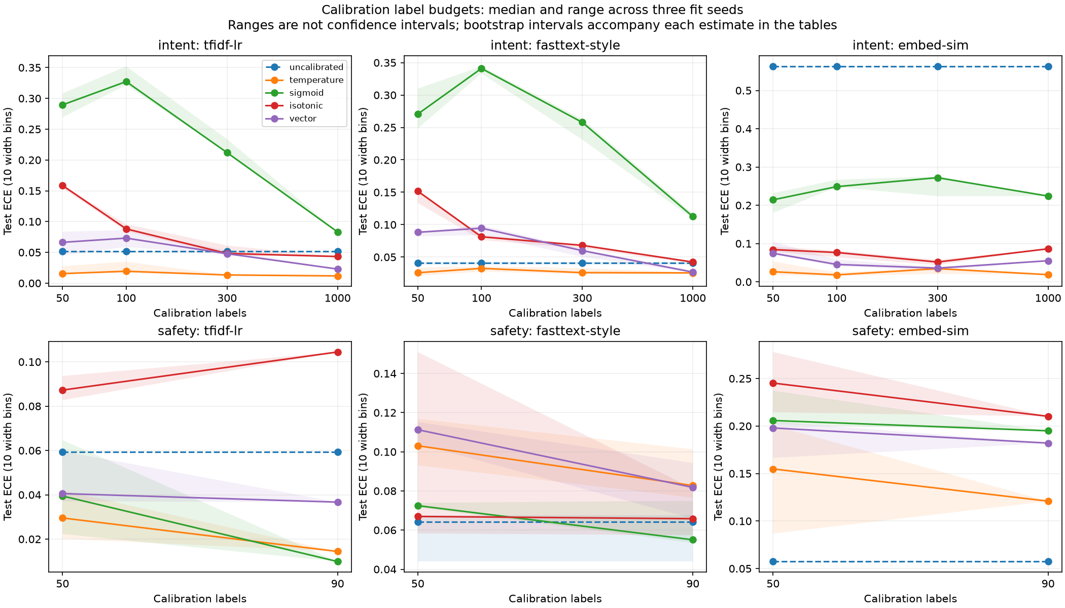
The complete table retains every budget, seed, wording and evaluated split, including losses and ties. The figure summarizes the same fixed fits; its shaded ranges across seeds are not confidence intervals.
OBSERVED, maximum-budget temperature minus raw, primary fit seed:
| Task | Provider | Metric | Difference [95% paired bootstrap] | n |
|---|---|---|---|---|
| intent | tfidf-lr | ece | -0.0402 [-0.0447, -0.0264] | 3080 |
| intent | tfidf-lr | brier | -0.0067 [-0.0096, -0.0035] | 3080 |
| intent | tfidf-lr | accuracy | 0.0000 [0.0000, 0.0000] | 3080 |
| intent | fasttext-style | ece | -0.0152 [-0.0305, -0.0000] | 3080 |
| intent | fasttext-style | brier | 0.0007 [-0.0016, 0.0032] | 3080 |
| intent | fasttext-style | accuracy | 0.0000 [0.0000, 0.0000] | 3080 |
| intent | embed-sim | ece | -0.5443 [-0.5500, -0.5223] | 3080 |
| intent | embed-sim | brier | -0.3867 [-0.4006, -0.3725] | 3080 |
| intent | embed-sim | accuracy | 0.0000 [0.0000, 0.0000] | 3080 |
| safety | tfidf-lr | ece | -0.0449 [-0.0703, 0.0268] | 116 |
| safety | tfidf-lr | brier | -0.0077 [-0.0315, 0.0152] | 116 |
| safety | tfidf-lr | accuracy | 0.0000 [0.0000, 0.0000] | 116 |
| safety | fasttext-style | ece | 0.0124 [-0.0442, 0.0726] | 116 |
| safety | fasttext-style | brier | 0.0014 [-0.0287, 0.0291] | 116 |
| safety | fasttext-style | accuracy | 0.0000 [0.0000, 0.0000] | 116 |
| safety | embed-sim | ece | 0.0636 [-0.0053, 0.0865] | 116 |
| safety | embed-sim | brier | 0.0181 [-0.0124, 0.0500] | 116 |
| safety | embed-sim | accuracy | 0.0000 [0.0000, 0.0000] | 116 |
Negative ECE/Brier differences favor the map; positive accuracy differences favor it. Read the interval, not only its sign. Full paired comparisons against raw and temperature, across every seed, budget, wording and test/shift condition, are retained in the evidence tables.
Temperature does not help every measured case. Safety fastText and embedding have higher test ECE and Brier point estimates after fitting. All three safety paired ECE and Brier intervals include zero. The small safety test cannot resolve those differences with these intervals. Intent fastText improves ECE while its Brier point estimate increases: even the direction depends on the measure.
OBSERVED, small-budget intent fits:
| Task/split | Provider | Method | Labels/seed/wording | ECE10 width [95% bootstrap] | Classwise ECE | Brier sum | Log loss | Accuracy | AUROC | n |
|---|---|---|---|---|---|---|---|---|---|---|
| intent/test | tfidf-lr | temperature | 50/0/w0 | 0.0155 [0.0115, 0.0274] | 0.0022 | 0.1768 | 0.4504 | 0.8779 | 0.9972 | 3080 |
| intent/test | tfidf-lr | isotonic | 50/0/w0 | 0.1591 [0.1501, 0.1711] | 0.0055 | 0.6515 | 2.8632 | 0.4581 | 0.8566 | 3080 |
| intent/test | tfidf-lr | temperature | 100/0/w0 | 0.0349 [0.0279, 0.0460] | 0.0022 | 0.1790 | 0.4722 | 0.8779 | 0.9972 | 3080 |
| intent/test | tfidf-lr | isotonic | 100/0/w0 | 0.0957 [0.0905, 0.1076] | 0.0042 | 0.4564 | 2.7424 | 0.6166 | 0.9216 | 3080 |
| intent/test | fasttext-style | temperature | 50/0/w0 | 0.0259 [0.0193, 0.0392] | 0.0026 | 0.2254 | 0.5707 | 0.8526 | 0.9963 | 3080 |
| intent/test | fasttext-style | isotonic | 50/0/w0 | 0.1533 [0.1438, 0.1664] | 0.0053 | 0.6682 | 3.1343 | 0.4571 | 0.8532 | 3080 |
| intent/test | fasttext-style | temperature | 100/0/w0 | 0.0326 [0.0268, 0.0458] | 0.0026 | 0.2243 | 0.5904 | 0.8526 | 0.9962 | 3080 |
| intent/test | fasttext-style | isotonic | 100/0/w0 | 0.0842 [0.0735, 0.0958] | 0.0040 | 0.4888 | 3.0462 | 0.6045 | 0.9140 | 3080 |
| intent/test | embed-sim | temperature | 50/0/w0 | 0.0175 [0.0155, 0.0340] | 0.0055 | 0.4358 | 1.2116 | 0.6799 | 0.9861 | 3080 |
| intent/test | embed-sim | isotonic | 50/0/w0 | 0.0842 [0.0695, 0.0973] | 0.0053 | 0.8055 | 4.8522 | 0.3558 | 0.7848 | 3080 |
| intent/test | embed-sim | temperature | 100/0/w0 | 0.0154 [0.0147, 0.0346] | 0.0054 | 0.4356 | 1.2117 | 0.6799 | 0.9861 | 3080 |
| intent/test | embed-sim | isotonic | 100/0/w0 | 0.0643 [0.0522, 0.0803] | 0.0059 | 0.6993 | 5.3657 | 0.4685 | 0.8491 | 3080 |
The LR subset at 50 labels leaves 38 classes unseen. Its isotonic map uses the declared constant fallback for those classes. This count is a measured limitation of the fitting evidence, not proof of a causal explanation for every observed accuracy change.
Primary-seed temperature wording ranges are intent/test: ECE 0.0176–0.0496, accuracy 0.5000–0.6799; safety/test: ECE 0.0924–0.1986, accuracy 0.4741–0.6983; safety/shift: ECE 0.0379–0.2447, accuracy 0.3740–0.6641. Each wording’s full-distribution scores, intervals and sample counts are in the retained tables. No wording was selected.
An ECE target can describe where these fits land. It does not authorize choosing a production budget or method from the test table. Such a choice needs a separate selection protocol and a new evaluation. The train-prior control remains in the results so a tiny ECE cannot masquerade as useful discrimination.
A conformal set is a different answer
PROPOSED recipe, taken from the documented split-conformal construction: the nonconformity score is one minus the raw probability assigned to the true label. We take the corrected order statistic from held-out calibration scores and include every candidate whose score is no larger. Ties remain together. If the required rank exceeds the calibration sample, the threshold is infinite. Empty sets are allowed and reported; we do not quietly insert a winning label.
This arm uses raw scores. It does not first fit a probability map on the same labels and then reuse them as though the score function were independent of the conformal calibration sample. That distinction protects the stated assumptions.
OBSERVED, maximum available budget, primary seed and wording, nominal coverage 0.90:
| Task/split | Provider | Labels | Coverage [95% bootstrap] | Mean set size [95% bootstrap] | Empty share | Singleton share | n |
|---|---|---|---|---|---|---|---|
| intent/test | tfidf-lr | 1000 | 0.9088 [0.8987, 0.9192] | 1.0955 [1.0844, 1.1062] | 0.0010 | 0.9081 | 3080 |
| intent/test | fasttext-style | 1000 | 0.9084 [0.8987, 0.9185] | 1.2545 [1.2344, 1.2744] | 0.0000 | 0.7977 | 3080 |
| intent/test | embed-sim | 1000 | 0.9166 [0.9068, 0.9253] | 6.1019 [6.0156, 6.1848] | 0.0003 | 0.0133 | 3080 |
| safety/test | tfidf-lr | 90 | 0.9310 [0.8793, 0.9741] | 1.1034 [1.0517, 1.1638] | 0.0000 | 0.8966 | 116 |
| safety/shift | tfidf-lr | 90 | 0.5687 [0.5076, 0.6221] | 1.0229 [1.0038, 1.0420] | 0.0000 | 0.9771 | 262 |
| safety/test | fasttext-style | 90 | 0.9569 [0.9224, 0.9914] | 1.1466 [1.0862, 1.2155] | 0.0000 | 0.8534 | 116 |
| safety/shift | fasttext-style | 90 | 0.5649 [0.5038, 0.6183] | 1.0344 [1.0153, 1.0573] | 0.0000 | 0.9656 | 262 |
| safety/test | embed-sim | 90 | 0.8793 [0.8190, 0.9397] | 1.6466 [1.5603, 1.7414] | 0.0000 | 0.3534 | 116 |
| safety/shift | embed-sim | 90 | 0.8550 [0.8092, 0.8969] | 1.8168 [1.7672, 1.8626] | 0.0000 | 0.1832 | 262 |
These are realized frequencies and conditional evaluation intervals. A finite test frequency below the nominal target is not, by itself, a refutation of the marginal theorem. The ordinary exchangeability guarantee is not available for this changed-source shift arm.
Safety embedding’s median coverage, 0.8793, narrowly misses the preregistered empirical floor of 0.88. Its primary-seed interval [0.8190, 0.9397] is wide. We retain the failed acceptance condition without turning that small miss into evidence against the marginal theorem.
Wrong: a calibrated probability and a conformal set offer the same guarantee.
Correct: probability maps are measured frequency claims; conformal sets have marginal coverage under stated assumptions. Neither promises this request is correct, and the set still needs an application policy.
The mean set size is part of the cost. A set containing every label can cover every outcome while resolving no decision. Coverage, singleton share, empty share and set size therefore travel together.
Evidence can become inapplicable
OBSERVED method: fit on the safety calibration distribution, then apply the same map and conformal threshold to the pinned safety shift dataset. This is a changed-source stress test, not elapsed-time measurement. Source, content and class balance change together; no causal explanation is isolated. There is no intent shift dataset in this experiment.
OBSERVED, safety temperature map fitted on A, then applied without refitting to B; primary seed, budget90:
| Provider | Shift minus test ECE [95% independent bootstrap] | Shift n | Test n |
|---|---|---|---|
| tfidf-lr | 0.3959 [0.2938, 0.4269] | 262 | 116 |
| fasttext-style | 0.2330 [0.1512, 0.2901] | 262 | 116 |
| embed-sim | 0.1238 [0.0213, 0.2061] | 262 | 116 |
You cannot infer a calendar expiry from this comparison. A date records when a fit happened. The dataset hash records which labeled scores supported it. Detecting a changed deployment distribution is another job; this chapter does not build a drift detector. A method that fails here is still a fitted method, but its provenance is not evidence of useful calibration on the shifted data.
The maps, running
Everything measured above used the book’s own providers, which are too large to check by eye. Here is the same machinery on a source small enough to understand: a seeded synthetic provider whose logits are deliberately three times too sharp, so it is overconfident by construction. Everything below is examples/ch10-calibration/walkthrough_ch10.py, which you can run as it stands. It uses no model and no downloaded data, and the output shows how the maps, the conformal sets and the evidence record behave. It says nothing about any real provider.
import hashlib
from pathlib import Path
import sys

import numpy as np

ROOT = Path(__file__).resolve().parents[2]
sys.path[:0] = [str(ROOT), str(ROOT / "src")]

from arbiter.calibration import CalibrationRecord, ProbabilityCalibrator, SplitConformal, scope_hash
from arbiter.contract import ChoiceQuestion
from benchmarks.harness import calibration as cal

K = 4
SHARPNESS = 3.0  # the source reports logits three times too sharp


def softmax(z):
    z = z - z.max(axis=1, keepdims=True)
    e = np.exp(z)
    return e / e.sum(axis=1, keepdims=True)


def draw(n, seed):
    """Labels and the overconfident source's probabilities for them."""
    rng = np.random.default_rng(seed)
    y = rng.integers(0, K, n)
    honest_logits = 1.2 * np.eye(K)[y] + rng.normal(0, 1, (n, K))
    return y, softmax(SHARPNESS * honest_logits)


def scores(y, p):
    return {"accuracy": float(np.mean(p.argmax(1) == y)), "ece": cal.top_label_ece(y, p), "brier": cal.brier_score(y, p)}


def main() -> None:
    y_cal, p_cal = draw(300, seed=1)  # the calibration split
    y_test, p_test = draw(5000, seed=2)  # held out, never used to fit

    # 1. Four maps, fitted on the calibration split and scored on the held-out one.
    print("1. an overconfident source, four maps fitted on 300 calibration items, scored on 5000 held-out")
    raw = scores(y_test, p_test)
    print(f"   {'raw':<12} accuracy {raw['accuracy']:.3f}  ECE {raw['ece']:.3f}  Brier {raw['brier']:.3f}")
    for method in ("temperature", "sigmoid", "isotonic", "vector"):
        fit = ProbabilityCalibrator(method).fit(y_cal, p_cal)
        s = scores(y_test, fit.transform(p_test))
        extra = f"  fitted temperature {fit.temperature:.2f}" if method == "temperature" else ""
        print(f"   {method:<12} accuracy {s['accuracy']:.3f}  ECE {s['ece']:.3f}  Brier {s['brier']:.3f}{extra}")

    # 2. How many calibration labels does each map need?
    print("2. calibration labels versus held-out ECE")
    print("   labels   temperature   isotonic")
    for n in (20, 100, 1000):
        y_n, p_n = draw(n, seed=10 + n)
        row = []
        for method in ("temperature", "isotonic"):
            fit = ProbabilityCalibrator(method).fit(y_n, p_n)
            row.append(cal.top_label_ece(y_test, fit.transform(p_test)))
        print(f"   {n:>6}   {row[0]:>11.3f}   {row[1]:>8.3f}")

    # 3. A conformal set is a different answer: a set of labels with a coverage guarantee.
    print("3. split conformal sets at alpha = 0.10")
    conformal = SplitConformal(alpha=0.10).fit(y_cal, p_cal)
    sets = conformal.predict(p_test)
    covered = float(np.mean(sets[np.arange(len(y_test)), y_test]))
    print(f"   one calibration split: coverage {covered:.3f}, mean set size {sets.sum(1).mean():.2f} of {K} labels")
    draws = []
    for seed in range(100, 200):
        y_d, p_d = draw(300, seed=seed)
        draws.append(float(np.mean(SplitConformal(alpha=0.10).fit(y_d, p_d).predict(p_test)[np.arange(len(y_test)), y_test])))
    print(f"   100 independent calibration splits: coverage mean {np.mean(draws):.3f}, lowest {min(draws):.3f}, highest {max(draws):.3f}")
    print("   the guarantee (at least 0.900) is on average over calibration draws; any one split can land below it")
    tiny = SplitConformal(alpha=0.10).fit(y_cal[:5], p_cal[:5])
    print(f"   with only 5 calibration items the quantile is {tiny.q}: every label goes in the set")

    # 4. The receipt: what the runtime can check about a fitted map.
    print("4. the evidence record")
    fit = ProbabilityCalibrator("temperature").fit(y_cal, p_cal)
    metrics = scores(y_cal, fit.transform(p_cal))
    metrics.update(log_loss=cal.clipped_log_loss(y_cal, fit.transform(p_cal)))
    question = ChoiceQuestion("q", "Which synthetic label?", {f"c{i}": None for i in range(K)})
    record = CalibrationRecord(
        "temperature", hashlib.sha256(y_cal.tobytes() + p_cal.tobytes()).hexdigest(), len(y_cal),
        "2026-10-08", metrics, tuple(f"c{i}" for i in range(K)), "synthetic-source",
        scope_hash(question), fit.digest(), "examples/ch10-calibration/walkthrough_ch10.py",
    )
    print(f"   method {record.method}, fitted on {record.n} items, labels {list(record.labels)}")
    print(f"   state: {record.state().kind.value}, evidence: {record.evidence}")
    other = hashlib.sha256(b"a different dataset").hexdigest()
    try:
        record.require_dataset(other)
    except ValueError as exc:
        print(f"   used on another dataset -> ValueError: {exc}")
1. an overconfident source, four maps fitted on 300 calibration items, scored on 5000 held-out
   raw          accuracy 0.612  ECE 0.207  Brier 0.578
   temperature  accuracy 0.612  ECE 0.020  Brier 0.510  fitted temperature 2.34
   sigmoid      accuracy 0.613  ECE 0.024  Brier 0.513
   isotonic     accuracy 0.614  ECE 0.043  Brier 0.520
   vector       accuracy 0.609  ECE 0.038  Brier 0.518
2. calibration labels versus held-out ECE
   labels   temperature   isotonic
       20         0.017      0.158
      100         0.008      0.042
     1000         0.008      0.040
3. split conformal sets at alpha = 0.10
   one calibration split: coverage 0.892, mean set size 2.11 of 4 labels
   100 independent calibration splits: coverage mean 0.903, lowest 0.870, highest 0.938
   the guarantee (at least 0.900) is on average over calibration draws; any one split can land below it
   with only 5 calibration items the quantile is inf: every label goes in the set
4. the evidence record
   method temperature, fitted on 300 items, labels ['c0', 'c1', 'c2', 'c3']
   state: CALIBRATED, evidence: examples/ch10-calibration/walkthrough_ch10.py
   used on another dataset -> ValueError: calibration evidence belongs to another dataset; re-evaluate
Read it part by part.
- A map fitted on 300 items fixes the held-out ECE and leaves the decisions alone. The raw source has an ECE of 0.207. Temperature scaling brings it to 0.020 with a single fitted number, 2.34, which is the sharpening it had to undo. Sigmoid, isotonic and the vector map reach 0.024, 0.043 and 0.038. Accuracy sits at about 0.61 throughout; the maps that can reorder classes move it by a few thousandths in either direction, while temperature cannot move it at all. This is the shape the chapter’s expectation predicted for a source with one simple defect, and it is exactly the case where the simplest map should win.
- The flexible maps need more labels. With 20 calibration items, temperature already reaches 0.017 while isotonic is at 0.158, only a modest improvement on the raw source’s 0.207 and nowhere near the one-parameter fit. By 100 labels isotonic is at 0.042 and stops improving, while temperature settles at 0.008. A map with many degrees of freedom has to be paid for with labels.
- A conformal set is a different answer, with a guarantee about averages. At alpha 0.10 one 300-item calibration split gives a coverage of 0.892, just under the nominal 0.900. That is not a bug. The guarantee is that coverage is at least 0.900 on average over calibration draws, and across 100 independent splits the mean is 0.903, ranging from 0.870 to 0.938. Any single split can land below the line. With only five calibration items the quantile is infinite, so every label goes into the set: the method refuses to promise anything it cannot back.
- A record is a receipt, not a certificate. It binds the method, the fitting data’s hash, the labels and the question scope, and the runtime can refuse to attribute it to a different dataset. It cannot say whether tomorrow’s requests resemble the 300 items it was fitted on.
Give the runtime something to check
PROPOSED: CalibrationRecord persists method, calibration-data hash, label
count, date and fit metrics. It also binds ordered labels, provider model,
question scope, parameter hash, seed and the evidence artifact. Import the
reason to persist identity and provenance from
Memory From First Principles, rather than treating a status
word as a memory of how the number was produced.
The new result view requires a record whenever it carries the calibrated state. The single-choice provider adapter checks the record against the fitted map, question and returned model. It attaches the record to each successful result. A typed provider refusal remains a refusal and carries no probability-calibration assertion. Earlier constructors and imports remain unchanged.
The adapter binds the returned model string, not a cryptographic identity of the provider’s weights. A revision changed under the same string could evade that check. It recomputes concentration from the transformed distribution; concentration still does not become the probability that the selected answer is correct.
This is a structural gate. CALIBRATED denotes a recorded fitted transformation,
not certification that a target was reached. Fit metrics are labelled as fit
metrics; held-out outcomes are in the evaluation record. The evidence reference
is necessary for a claim but cannot make a false reference true. The explicit
dataset-identity check rejects attributing one dataset’s record to another;
it does not detect distribution shift from an arbitrary incoming request.
OBSERVED: 99 calibration and contract tests pass. Independent checks cover sigmoid/isotonic library references, a second scalar optimizer, vector/sigmoid gradients, separable binary and multiclass fixtures, replay serialization, missing-class behavior and a conformal exchangeable-rank oracle. A planted uncorrected rank fails the quantile fixture; seeded missing or mismatched records are rejected. Earlier version-2/version-3 contract tests still pass. Full real NLI/model arms were not rerun.
Run the offline synthetic demonstration:
python examples/ch10-calibration/demo_ch10.py
Its scores illustrate the adapter, not benchmark performance. The source example README gives the staged replay commands and the read-only verifier. Fitted maps and records are committed, so replay does not need to refit them or call a model.
What Arbiter-1 has earned
OBSERVED, preregistered outcomes:
These acceptance conditions use medians across the three fit seeds, as registered. The main tables display seed 0. Neither view selects the most favorable seed.
- P1, temperature with 100 labels: tfidf-lr: SUPPORTED, gain 0.0326 versus full-budget gain 0.0402; fasttext-style: REFUTED, gain 0.0082 versus full-budget gain 0.0152.
- P2: SUPPORTED. The isotonic small-budget penalty was tested across all three intent providers.
- P3: REFUTED. Vector versus temperature used the fixed alternative and penalty, not full Dirichlet.
- P4: REFUTED. The empirical coverage-and-size prediction was checked for every provider and task.
- P5: SUPPORTED. Temperature ECE changes and raw conformal coverage were checked on safety shift.
- P6: SUPPORTED. The runtime rejects the seeded evidence omissions and binding mismatches.
The isotonic small-budget penalty holds for LR and fastText, while embedding is a counterexample to a universal version. Vector scaling misses the declared ECE advantage for all three providers. Its better intent embedding Brier and accuracy do not change that preregistered ECE verdict.
PROPOSED conclusion: start with the low-capacity map as a measured baseline, retain evidence when more complex maps lose, and carry the complete record into the runtime. Arbiter-1 earns an evidence-bearing calibration layer here, not a claim that every transformed score is reliable or that one method is best for deployment. No global H1/H3 verdict or Chapter 7 pivot ruling follows.
The research readings are partial. Platt’s original was read from rendered pages, not the secondary lecture file. Appendix algorithms and detailed supplements were not audited. Safety label budgets remain limited, and shared public test items have been examined in earlier chapters. Conditional bootstrap intervals and three fit seeds do not turn those items into new independent datasets.
Hosted Jev, NLI and option-scored model calibration are NOT_OBSERVED here. No hosted cache existed. Vendor documentation still describes confidence as a concentration statistic; the HN allegations remain commenter claims. TypeSafe confidence documentation. Third-party AnyJev calibration is adjacent prior art, not a substitute for our absent hosted measurement. AnyJev.
Fit CPU time, wall time and peak traced Python allocations are recorded. Those allocations are not full process RSS, and serving latency was not measured. There is no accuracy-cost-latency Pareto verdict. No source in this chapter makes a provider’s internal mechanism observable through its calibration behavior.
Arbiter-1 is the provisional provider plus its fitted map and calibration evidence. What is its calibration evidence, and when does it expire? The next chapter, Abstain, has to choose what your program does when that evidence cannot justify an automatic action.