Next-Token Loss and Teacher Forcing
Derive stable next-token cross-entropy, check a numerical reference, and apply the objective to the exact labels and masks from Chapter 07.
A training run reports a lower loss after a change to its data loader. The model may have become better at predicting the intended answers. The loader may instead have started supervising easy prompt tokens, counted padding as an answer, or divided by a larger denominator. A scalar cannot tell us which event occurred. We need to know the probability being scored, the positions included and the reduction used.
Chapter 07 constructed a batch with seven supervised targets. We will consume that same batch, without redefining its token IDs or masks, and calculate exactly what its loss means. The calculation comes before optimisation: at this stage an array of logits is enough. We do not need to train a model to verify the objective it would receive.
From a sequence probability to local predictions
For a sequence $x_0,\ldots,x_{T-1}$, the probability chain rule gives
At each position the model returns one real-valued logit per vocabulary entry. A logit is an unnormalised score. It can be negative or positive, and it is not itself a probability. Let $z_{t,v}$ be the logit at position $t$ for vocabulary entry $v$. Here $t$ indexes the logit position; its next-token target comes from sequence position $t+1$. Softmax converts those scores to a distribution:
For a target ID $y$, the negative log-likelihood is
Cross-entropy between a target distribution $q$ and a predicted distribution $p$ is $-\sum_v q_v\log p_v$. For an observed next token, the target distribution places probability one on its ID and zero elsewhere. The sum then reduces to $-\log p_y$. This equivalence explains why integer class targets can implement the same objective without constructing a large one-hot target tensor.
Calculate two predictions by hand
Consider the following artificial logit table. These scores are chosen inputs to the calculation, not outputs attributed to a trained model.
| Prediction | Logits for IDs 0, 1, 2 | Correct ID |
|---|---|---|
| First | 2, 1, 0 | 0 |
| Second | 0, 2, 1 | 2 |
For the first prediction, centre the scores on their maximum, 2. Its normalising sum becomes $1+e^{-1}+e^{-2}$, and the correct entry has centred score zero. Therefore
The reference uses math.fsum for the exponential sum. It explicitly rejects non-finite inputs, malformed targets and an empty set of scored positions. It remains small enough to inspect independently of PyTorch’s loss implementation.
Stabilise the calculation without changing the objective
Computing exp(10002) directly can overflow, even though logits 10002, 10001 and 10000 describe the same distribution as 2, 1 and 0. Let $m=\max_v z_v$. Then
No rearrangement rescues information already lost when logits were represented with insufficient precision. Two distinct scores can round to the same FP16 value before the loss sees them. Chapter 10 will separate representation precision, loss precision and gradient scaling. Here the numerical reference uses float64; the shared loss promotes FP16 or BF16 input logits to FP32 for its cross-entropy calculation, while leaving float64 inputs in float64.
The implementation uses the library’s fused cross-entropy operation rather than applying softmax, taking its logarithm and then selecting the target in separate low-precision steps. The PyTorch cross-entropy interface documents the integer-target and ignored-index API; measured behaviour in this book is pinned to PyTorch 2.6.0 rather than inferred from the current documentation version.
Teacher forcing is a conditioning choice
During this training calculation, the input contains the recorded previous tokens. At the position predicting K in our OK answer, the preceding input contains the recorded O. We do not first ask the model to generate an O and then replace the input with whatever it happens to produce. Supplying the recorded history is teacher forcing.
This permits predictions at many positions to be computed together. It does not permit a position to attend to the token it is supposed to predict or to later tokens. The causal attention restriction maintains that separation. Parallel evaluation of many conditional factors is compatible with an autoregressive factorisation.
At generation time, the model instead conditions on its own previously selected outputs. A model can therefore have a modest teacher-forced loss yet perform poorly after making an early generation error. Training and generation also differ in the role of sampling, stopping rules and the availability of the correct history. This chapter does not measure that gap with a real language model; the capstone will report autoregressive outputs separately from teacher-forced loss on a tiny educational model.
Apply one shift to the existing batch
Our model interface will return logits at every input position, with shape $B\times T\times V$. The target stored at label position $t$ is predicted from logit position $t-1$. The shared loss owns the shift:
scores = logits[:, :-1, :]
targets = labels[:, 1:]
For Chapter 07’s first row, logit position 6 predicts label 7, the ID for O; logit 7 predicts K; logit 8 predicts the assistant ending. The last logit has no following label in the supplied sequence. The initial label is ignored because no preceding logit is supplied for it.
The shared function requires that initial label to be -100, checks the tensor shapes and vocabulary range, and rejects NaN or infinite logits. These are useful diagnostics for an educational interface. They are not a universal rule that every external framework must expose the same arrays. Some model forward methods perform the shift internally. In that case pass unshifted labels to the model, and do not also apply our external shift to its already-computed loss.
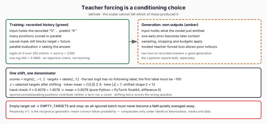
The two panels contrast what the model conditions on: recorded history during training against its own outputs during generation. The strip below fixes the shared mechanics — one shift, the seven-target denominator with its checked arithmetic — and the guard refuses an empty target set instead of averaging it away.
Shifting twice changes the question. An output conditioned on the assistant marker would be scored against K rather than O. Our non-uniform-logit regression makes this error visible: logits that strongly favour the correctly aligned next tokens have a small loss, while the deliberately misaligned targets produce a much larger one. Uniform logits alone cannot reveal the error because every target has the same probability.
Define the scored positions and denominator together
Let $J$ be the set of selected target positions after the causal shift. The token-mean objective is
Sequence means introduce a different weighting. If one example has two targets and another has one, the mean of their two sequence means gives equal weight to the examples. A token mean gives the first example twice the weight. Neither statistic is inherently dishonest, but changing between them changes the objective. The shared implementation sums all selected token losses and divides once by their total count.
That distinction will also matter for gradient accumulation. Dividing each microbatch mean by the number of microbatches is equivalent to a token mean only when their target counts match. An exact accumulated token mean instead weights every microbatch by its share of the total selected targets.
For this numerical probe we use the unmerged byte/control alphabet with 262 entries. The earlier worked batch contains only those original IDs, even though Chapter 07 also inspected an encoder with additional learned merges. We preserve the supplied IDs and masks; we do not claim that this smaller output vocabulary covers every merged token. The capstone binds an explicitly unmerged tokenizer.
For a direct numerical check, assign all 262 logits the value zero at every position in the exported two-row batch. Each selected target then has probability $1/262$, giving a derived loss of $\log262$. The CPU reference run measured:
| Quantity | Observed value |
|---|---|
| Valid targets after shifting | 7 |
| Per-token mean | 5.568344503761097 |
| Sum | 38.978411526327676 |
| Shifted target shape | $2\times12$ |
| Gradient norm at an ignored prediction position | 0 |
The same tiny calculation executed on CUDA. It is an objective check, not a claim that the uniform predictor has learned anything. Adding ignored padding leaves the scalar loss unchanged, and the tests verify zero gradients at ignored prediction positions and at the unused final logit.
Refuse a batch with no objective
If $J$ is empty, the mean divides by zero. An all-ignored batch can arise when truncation removes the answer, the loss mask selects the wrong role, or filtering creates an empty target set. Returning a NaN and hoping that the optimiser or loss scaler will repair it hides the actual problem.
The shared function reports EMPTY_TARGETS before calling a mean reduction. Training code must decide whether an empty example should be rejected, deliberately excluded with a recorded count, or prevented by a different truncation policy. That decision belongs to data preparation. It should not silently change which dataset was trained.
A batch can also contain a valid target outside the declared vocabulary. That is a different error, reported as TARGET_RANGE, and often indicates a tokenizer/model mismatch. A shape mismatch points to a different layer again: labels from one serialisation may have been paired with IDs from another. Specific diagnostics preserve the distinction between no objective, an impossible ID and an alignment error.
Read perplexity with its conditioning assumptions
For a token-mean negative log-likelihood $L$, perplexity is $e^L$. It is the reciprocal geometric mean of the probabilities assigned to the selected correct tokens. A uniform distribution over $V$ entries has perplexity $V$, directly from $e^{\log V}=V$.
Perplexity is meaningful only with its tokenisation, target selection and data distribution specified. Changing the vocabulary changes what a token represents. Changing an answer-only mask to an all-text mask changes the set being averaged. Comparing those resulting scalars without qualification does not isolate a model improvement.
Even a correctly computed lower answer loss does not establish correct routing, valid JSON, grounded citations, safe abstention or acceptable latency. Those are separately declared task properties. The objective rewards probability on recorded target sequences; it cannot decide whether the records are true, current or representative. The incident-triage task’s evaluation requirements remain separate from this educational exercise.
The companion example now turns the exact token batch into a scalar with a known denominator, a verified numerical reference and an explicit alignment. Chapter 09 follows that scalar backwards through an actual small Transformer. Its question is no longer which prediction was penalised, but how that penalty reaches each trainable parameter.
Further Reading
- Samy Bengio et al., “Scheduled Sampling for Sequence Prediction with Recurrent Neural Networks” (2015). Read the source. The classic statement of the exposure-bias gap between teacher-forced training and free-running generation that the chapter keeps separate.
- PyTorch contributors, “torch.nn.functional.cross_entropy” (PyTorch 2.6 documentation). Read the source. Documents the fused operation behind the chapter’s shared loss, including the -100 ignore convention and the absence of shifting.
- Ian Goodfellow, Yoshua Bengio and Aaron Courville, “Deep Learning”, Chapter 5: Machine Learning Basics (2016). Read the source. The probabilistic foundation for the one-hot reduction: negative log-likelihood as maximum likelihood with test-set performance as the target.