Designing a LoRA Experiment
Turn adapter settings into identifiable paired experiments, distinguish training mechanics from quality, and reject incomplete evidence.
One rank-two adapter finishes with a lower loss than a rank-one adapter. Should we use rank two? The answer depends on what changed, which loss was measured, how the runs were paired and what the experiment was designed to establish. A single successful configuration does not answer those questions.
LoRA exposes several choices: rank, scaling, target modules, dropout and the surrounding optimiser and data protocol. Their interactions make casual experimentation easy and interpretation difficult. A useful experiment begins with a question small enough that its observations can distinguish plausible answers.
The executed experiment here is deliberately limited. Four tiny CPU runs vary rank at fixed alpha/r over two seeds. They report training histories and resource state, perform no configuration selection and make no pretrained-model claim. The real-model matrix remains planned pending its separate gates.
State the estimand before choosing a grid
An estimand is the quantity the experiment intends to learn about. “Does LoRA work?” is too broad. “At this checkpoint, data distribution and compute budget, what is the paired change in approved task performance when rank rises from eight to sixteen at fixed scaling?” is closer to an executable question.
That wording fixes many otherwise ambiguous choices. It names the base, data, budget, outcome and intervention. It also exposes missing evidence: without approved evaluation data and a valid scorer, the proposed performance difference cannot yet be measured.
Our tiny CPU question is narrower: how do final training losses differ after six updates when rank changes from one to two at fixed alpha/r, target module, fixtures, learning rate and update count? This probes the experiment harness and adapter mechanics. Training loss on two character pairs is its outcome, not incident quality or a generalisation estimate.
A rank comparison can answer a different question at fixed time rather than fixed updates. A larger rank may have more capacity but fewer updates within the same wall-clock budget. Neither design is inherently wrong. Mixing them without naming the budget changes the estimand.
Separate the intervention from the controlled context
Let a run configuration be
A controlled rank comparison fixes the other relevant choices or explicitly models their interaction. Increasing rank while keeping alpha fixed changes alpha/r. Moving from query/value to all linear modules changes both placement and parameter count. Increasing epochs on a duplicated dataset changes update exposure without necessarily adding independent information.
The implemented matrix fixes alpha/r at two: rank one uses alpha two, and rank two uses alpha four. Both target only blocks.0.project in the tiny Transformer, use dropout zero, learning rate 0.02, microbatch one and six updates. The context limit is sixteen positions.
These settings differ from Chapter 21’s standalone rank-two, alpha-two mechanism run. Its history is not an additional controlled rank observation. Each report retains its configuration so a superficially similar run cannot enter the wrong comparison.
Use seeds as paired experimental conditions
A seed affects random base initialisation, adapter factors and potentially dropout or data order. Repeating the same seed can verify deterministic replay. It does not create a second independent experiment.
For a paired rank comparison on seed s, both ranks begin from the same tiny base. They then receive their declared adapter initialisations. The higher-rank model has more factor entries, so “same seed” does not mean every trainable random number is identical between ranks. Pairing still removes the change in base initialisation as an uncontrolled difference.
The matrix uses seeds 37 and 38. The configuration is hashed into a run identity;
changing seed, rank, alpha or another declared value changes that identity.
The report builder verifies the adapter manifest rather than trusting a run
label: the manifest configuration must equal the planned seed, rank, alpha,
steps, learning rate and microbatch; its digest must recompute; and its base
digest must equal the planned seed’s base. An observation carrying another
run’s manifest fails EXPERIMENT_BINDING before a paired difference is formed.
The four observed final training losses are:
| Seed | Rank | Alpha | Final training loss | Trainable parameters |
|---|---|---|---|---|
| 37 | 1 | 2 | 5.526040 | 16 |
| 37 | 2 | 4 | 5.513657 | 32 |
| 38 | 1 | 2 | 6.420136 | 16 |
| 38 | 2 | 4 | 6.368772 | 32 |
Rank two has a lower final training loss in both pairs. The paired differences, higher rank minus lower rank, are approximately -0.012383 and -0.051364.
Those are descriptive results from the specified tiny problem. They do not establish that rank two is optimal, that either adapter generalises, or that a Qwen model would show the same difference. The different base losses across seeds also illustrate why an unpaired single-run comparison can be misleading.
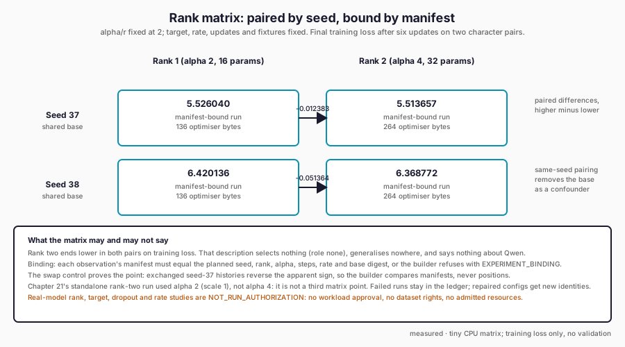
The matrix pairs ranks through their shared base and binds each cell to its manifest. Notice that both differences favour rank two on training loss while the selection role stays none — no winner is declared and no interval is drawn from two seeds.
Keep the measured outcome distinct from the selection outcome
The CPU report contains training-loss histories only. It does not measure a validation score, choose a winner or inspect protected incident examples. Its selection role is explicitly none. Future selection is restricted to an approved validation boundary.
This distinction matters even when the experiment matrix already names validation as the eventual selection role. A declared future policy is not a measured validation result. Labelling a training loss “validation” would not change the data that produced it.
A useful eventual report separates at least three observations: optimisation behaviour on training examples, model selection using permitted validation evidence, and a confirmatory comparison under an approved final protocol. A run can succeed at the first and fail at the other two.
The engineering incident set also has no untouched protected benchmark. All examples have been inspected, and its capacity audit requires strong simple controls. Creating a new directory named final_test would not undo those facts.
Reject incomplete matrices before building a conclusion
The report builder requires every planned run exactly once. A missing run is EXPERIMENT_INCOMPLETE, not an invitation to average the survivors. Duplicate identities are also refused.
For each tiny observation it requires the declared CPU/random-model scope, finite loss history, an unchanged frozen base and exact adapter reload. A test-selected or pretrained-model-labelled observation cannot be substituted for this matrix’s fixture evidence.
These checks prevent common bookkeeping failures. They do not authenticate a maliciously invented report or provide a trusted execution service. Source digests, environment observations and recorded commands make the runs inspectable; production-grade receipts remain an open boundary.
The negative control is concrete. Swap the rank-one and rank-two histories of
seed 37, including their adapter manifests, and the report builder must refuse.
The naive builder would recompute a positive seed-37 difference, reversing the
apparent sign of the rank effect. The repaired builder compares each
observation’s manifest configuration with the planned run and checks the recorded
base digest, so the swap never reaches the comparison. A matrix with more than
two ranks is paired explicitly: every higher rank is compared with the lowest
rank in the same seed, and both ranks are labelled in the output. A matrix that
cannot form a pair raises EXPERIMENT_DESIGN instead of returning an empty list.
Failed runs belong in the experiment ledger. If a configuration exceeds memory, produces nonfinite gradients or fails reload, that is evidence about the proposed method under its constraints. Reporting only configurations that finish creates a survivor bias, especially when the selection question concerns reliability.
A repaired configuration needs a new identity. Reducing sequence length after an out-of-memory error can be a reasonable next experiment, but it is not the original run finally passing.
Analyse uncertainty at the level actually sampled
For S paired conditions, let d_s be the higher-rank outcome minus the lower-rank outcome. The paired mean is
A future task comparison has at least two uncertainty sources: training randomness and the evaluation sample. Repeating seeds does not compensate for one base incident per class. Repeating the fixed-prefix surface does not add an independent incident. A statistical protocol needs to explain which source it samples and which groups remain dependent.
Paired incident comparisons can reduce avoidable variation when both methods see the same cases. Group-aware resampling can preserve declared family dependencies. Neither procedure creates semantic diversity absent from the data. If a class or severity has no support, the corresponding estimate remains unestablished.
The current report therefore provides the raw paired differences and an explicit uncertainty limitation rather than an impressive-looking confidence band.
Vary targets with a separate question
Rank and target placement affect different parts of the hypothesis space. An adapter on a query projection changes how attention is formed; one on a value or output projection changes a different transformation. MLP targets provide another intervention. Their names and actual shapes must be checked in the selected architecture.
Comparing the same rank across different target sets does not hold trainable parameter count constant. Comparing equal counts may require different ranks. A good design chooses which resource or capacity quantity matters to the question and reports the others.
Biases, embeddings and the language-model head are additional choices. A library option that leaves one of them trainable can dominate the adapter ledger or introduce a new learning path. A trainable-parameter dump and a before/after base hash are more informative than a configuration label alone.
For the tiny mechanism we keep one exact target and expose its count. A real-model target ablation remains a proposed experiment until the model, dataset and resource gates are satisfied.
Treat optimiser and data choices as potential confounders
Learning rate, update count and effective batch influence how much opportunity each adapter has to learn. A larger rank may need a different rate or regularisation, but tuning only that rank more extensively would change the comparison budget.
Gradient accumulation also requires the correct loss weighting from Chapter 21. A change in answer lengths can alter token exposure even when the number of sequences per update is fixed. Context truncation can remove targets or change conditioning information.
Data quality is not merely another scalar grid axis. Correcting a label, changing the policy or altering a split changes the dataset/study identity. Such a comparison can be valuable, but it is a cross-revision study rather than a hyperparameter tweak.
The current 0.2.1 incident set mandates class-frequency, metadata-only, train-only lexical and deterministic controls. Its 60% metadata control and perfect lexical family-challenge control must accompany any eventual authorised model comparison. A rank effect cannot be interpreted sensibly while those explanations are hidden.
Plan cost and negative results before execution
A candidate configuration has several resource costs: base storage, adapter parameters, gradients, optimiser moments, activations and temporary runtime state. Rank affects some of these directly and others indirectly through implementation.
In our tiny matrix, rank one has sixteen trainable parameters and 136 bytes of optimiser tensors; rank two has thirty-two and 264 bytes. The counts include the implementation’s scalar step state. They do not measure a whole model’s process memory or GPU throughput.
The future model matrix should have a total run budget, per-run ceiling, stop conditions and a rule for incomplete evaluation. If the necessary comparison cannot be completed, the correct result is experiment pending or insufficient evidence, not a selected winner.
An observed negative result can support a useful decision. If larger rank adds cost without a defensible quality benefit, a smaller adapter or no training may be preferable. Our current tiny training-loss result is not sufficient to make that operational decision.
Reproduce the matrix and retain its identity
The matrix and report builder live in ftlab.adapters.protocol. The CPU batch writes matrix.json beside each run’s configuration, histories and adapter identity. Fresh output directories prevent replacement of earlier results. Repeated execution under the same pinned environment verifies deterministic fixture results separately from the scientific interpretation.
Real pretrained-model rank, target, dropout and learning-rate studies are NOT_RUN_AUTHORIZATION. They need explicit workload approval, dataset rights, fresh resource admission and an evaluation protocol capable of measuring the claimed effect. Passing a matrix-shape check does not satisfy those prerequisites.
One remaining intervention changes the stored base itself. Quantising it can reduce memory while leaving the adapter trainable, but it introduces a second source of approximation and backend dependence. Chapter 24 separates those changes before asking what a QLoRA comparison could establish.
Further Reading
- Edward J. Hu et al., “LoRA” (2021). Read the source. Ablates rank and placement under shared training conditions, modelling controlled intervention design; also recommended in Chapters 21 and 22 for identity and algebra.
- Tim Dettmers et al., “QLoRA: Efficient Finetuning of Quantized LLMs” (2023). Read the source. Compares many finetunes across data and models, showing why quantisation, data and budget need matched controls.
- Sayash Kapoor and Arvind Narayanan, “Leakage and the Reproducibility Crisis in ML-based Science” (2022). Read the source. Catalogues how test-driven selection leaks, supporting validation-only selection; also recommended in Chapter 17 for split leakage.