The Memory and Compute Budget
Measure a real small Transformer step, reconcile tensor storage with analytical estimates, and distinguish allocator peaks, saved tensors and useful throughput.
A model’s parameter arrays occupy less than a megabyte, yet a CUDA measurement reports tens of megabytes allocated. The discrepancy need not indicate a leak. A training step contains gradients, moment estimates, saved forward values and temporary workspace, and the runtime may retain storage for later reuse. To understand a measurement, we must specify both what it counts and where its interval begins.
Chapter 04 estimated resource requirements before execution. Here we reuse its arithmetic where the assumptions match and compare it with actual tensors from our shared Transformer. We are measuring runtime mechanisms, not revisiting the financial case for adaptation or certifying that a future language model fits on the same GPU.
Count stored elements before estimating invisible work
A dense tensor’s logical byte count is its element count multiplied by the element size. A shape $3\times4$ tensor has twelve elements, so FP32 storage contributes 48 logical bytes and FP64 contributes 96. A view can share the same underlying storage with another tensor. Adding both logical sizes would then double-count physical storage.
Our small Transformer deliberately uses separate token embeddings and output weights. Its parameter count can be derived independently of the module enumeration. For vocabulary $V$, width $d$, MLP width $f$, context capacity $T_{\max}$ and $n$ blocks, the implemented count is
At $V=262$, $d=32$, $f=64$, $T_{\max}=32$ and one block, it gives 26,400 parameters. Runtime enumeration agrees. With all parameters trainable in FP32, the measured logical arrays are:
| Category | Logical bytes |
|---|---|
| Parameters | 105,600 |
| Gradients after backward | 105,600 |
| Adam first and second moments | 211,200 |
| Seventeen FP32 step-counter tensors | 68 |
| Total of these categories | 422,468 |
Before the first step, the Adam state is allocated lazily and contributes zero. Clearing gradients to None also removes their current tensor buffers from this logical ledger. The allocator may retain the released storage, so that change does not imply that all corresponding GPU reservation is returned to the driver.
The tested CUDA optimiser keeps the 68 step-counter bytes on the CPU and the two moment arrays on the GPU. A total across all optimiser tensors is therefore not automatically a GPU-only total. The report records state sizes by device rather than hiding that placement.
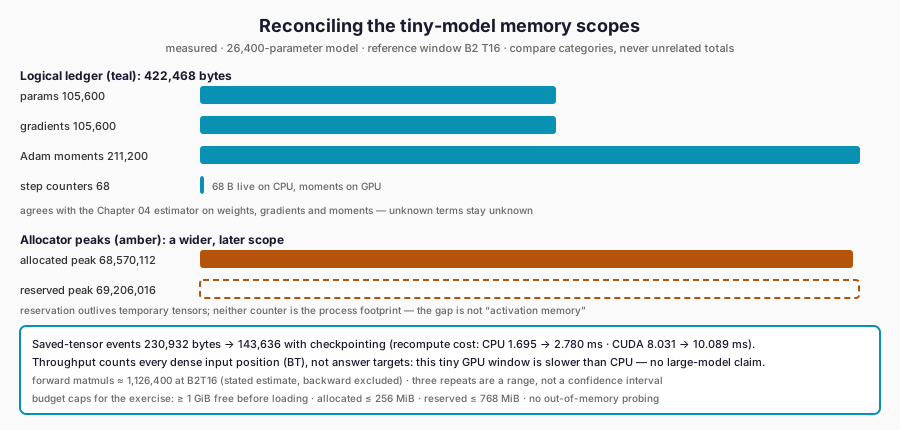
The figure separates the three scopes the section warns against mixing: the logical tensor ledger, the wider allocator peaks, and the saved-tensor event counts that change under checkpointing. The gap between the 422,468-byte ledger and the ~69 MB peaks is a difference of scope and timing, not an identified activation allocation.
Reconcile only terms with compatible assumptions
We pass the observed parameter count to Chapter 04’s existing estimator, using full FP32 updates and two FP32 optimiser state arrays. It predicts 105,600 weight bytes, 105,600 gradient bytes and 211,200 moment bytes. Those terms agree exactly with the measured corresponding tensors.
The extra 68 scalar-counter bytes are outside that two-array approximation. More importantly, the estimator still leaves activation, workspace and allocator assumptions unspecified. Agreement on weights and moments does not fill in those unknown terms or turn a lower bound into a complete device-memory prediction.
This is why we compare categories rather than subtracting unrelated totals and calling the residual an error. The analytical estimate describes selected arrays. A CUDA peak can include additional allocations live at a particular instant. A driver-level free-memory reading has a wider boundary still. Each can be useful without being interchangeable.
The old Qwen3 stored-versus-logical parameter discrepancy remains unresolved. Counting this tiny model’s actual tensors does not inspect Qwen’s weight files, tied storage or loader behaviour. We have not downloaded those weights or converted the earlier estimate into a measured model count.
Understand what backward keeps alive
Backward needs selected values from the forward computation. A linear map may need its input and weight; a nonlinearity may need an input or output; attention needs information sufficient for its matrix and softmax derivatives. These saved values depend on the actual implementation, whether gradients are required and which operations are fused.
The instrumentation uses saved-tensor hooks to count the logical size of values handed to autograd’s save mechanism. It returns detached views sharing the same values, without changing their numerical content. The resulting count is a count of save events and references, not a deduplicated live-memory peak. An already-counted parameter can be saved again, and different saved tensors can share storage.
At batch size 2 and sequence length 16, the reference recorded 230,932 logical saved-tensor bytes per measured repeat. That number is useful for comparing this instrumented computation with another configuration under the same hook policy. It is not a claim that backward exclusively allocated exactly that many new physical bytes.
Tracing every intermediate gradient, as in Chapter 09, also changes lifetime and memory use. The runtime measurement disables that teaching trace. Otherwise we would be measuring an instrumented diagnostic graph while describing it as the normal training path.
Separate allocation, reservation and device-wide availability
CUDA allocator statistics distinguish storage currently allocated to active allocations from storage reserved by the caching allocator. Reservation includes memory available for reuse within that allocator. Its peak can remain above the current allocated value after temporary tensors disappear.
Neither statistic is the total physical footprint of the process. CUDA context state, libraries, driver activity and other applications have their own costs. The PyTorch CUDA memory notes explain the allocator distinction; this experiment records the counters from the pinned runtime.
In one recorded window at batch 2 and length 16, peak allocated memory was 68,570,112 bytes and peak reserved memory was 69,206,016 bytes. Those totals are much larger than the parameter/gradient/moment ledger. The measurement starts after a warm-up that has already established library and optimiser state, and the baseline allocation is recorded separately.
It would be wrong to label the difference from 422,468 bytes as uniquely identified activation memory. Some workspace and persistent allocations can overlap with that boundary, and the counters do not give us an exhaustive owner-by-owner decomposition. Likewise, subtracting reservation from a device-wide free-memory reading would mix scopes and time points.
The run checks available memory before allocating its educational model and requires at least one GiB free. It caps allocated memory at 256 MiB and reservation at 768 MiB. These conservative bounds are far above the observed tiny workload but below the hardware’s full capacity. No out-of-memory crash is used as an experimental probe.
Measure a complete, warmed step
The timed window includes gradient clearing, forward computation, the selected loss, backward and an AdamW update. It excludes model construction and performs one warm-up step first, so lazy optimiser state and initial kernel setup are not mistaken for steady step costs. Three subsequent steps are timed individually.
CUDA operations can be queued asynchronously. Measuring only how long Python takes to enqueue them is not an execution-time measurement. We synchronise before starting the timer and after the step before stopping it. The CUDA timing guidance supplies the background for this boundary.
The reported tokens-per-second numerator is $BT$: every dense input position processed, including any padding and control markers. It is not the count of supervised answer targets, and it is not generated tokens per second. In these particular windows all rows have their chosen full length; only three target positions per row are supervised.
One final-code set of reference medians was:
| Batch | Length | CPU median, ms | CUDA median, ms | CUDA dense tokens/s |
|---|---|---|---|---|
| 1 | 8 | 1.365 | 9.200 | 870 |
| 2 | 8 | 1.474 | 7.116 | 2,248 |
| 2 | 16 | 1.695 | 8.031 | 3,984 |
| 4 | 16 | 1.809 | 6.952 | 9,206 |
| 2 | 32 | 1.701 | 6.386 | 10,023 |
These are small workloads under validation and hook instrumentation on the reference host. The GPU is slower in these complete windows. Dispatch, synchronisation, validation and Python overhead have substantial weight when the numerical work is this small. This does not predict how a large pretrained model, a fused implementation or a longer sequence would compare.
The non-monotonic medians are also a warning against over-reading three samples. The raw minimum, maximum and individual durations are retained, and a separate run showed timing variation. We do not turn three neighbouring measurements into a confidence interval, sustained hardware throughput or a promise that doubling a sequence makes the GPU faster.
Derive the main matrix-operation costs
For a dense matrix multiplication with dimensions $m\times k$ and $k\times n$, the usual approximation counts a multiply and addition as two operations, giving about $2mkn$ FLOPs. It omits details such as edge terms, data movement and kernel scheduling.
Under that convention, our forward matrix products cost approximately
At batch 2 and length 16, the formula gives 1,126,400 forward matrix FLOPs. One stored per-head score array has $nBhT^2=1,024$ elements, or 4,096 FP32 bytes. That is one array, not the complete attention-memory requirement.
Doubling sequence length doubles several linear terms but quadruples the dense attention-score element count. Real implementations may avoid storing the full matrix or fuse operations, so this formula is an explanation of the visible educational code. It should not be used as a universal allocation formula for every attention kernel.
Execution time depends on moving bytes as well as on arithmetic. Small operations can be launch-limited; larger operations may become bandwidth- or compute-limited. The ratio of FLOPs to bytes moved, kernel efficiency and the degree of parallelism all matter. Our timing window is too small and too instrumented to diagnose a particular hardware bottleneck conclusively.
Trade recomputation for saved values
Activation checkpointing discards selected saved intermediates and recomputes them during backward. Our optional block path uses the non-reentrant checkpoint interface explicitly. A regression checks matching outputs and gradients against the uncheckpointed computation with dropout disabled.
At batch 2 and length 16, the logical saved-event count fell from 230,932 to 143,636 bytes. CPU median step time rose from approximately 1.695 to 2.780 ms in the reference windows; the CUDA medians were approximately 8.031 and 10.089 ms. The hook totals are not a statement of equivalent VRAM savings, but the extra computation is visible in the measured step boundary.
When stochastic operations are present, recomputation also needs consistent randomness. Other side effects can make re-execution inappropriate. Checkpointing is therefore a change to how the graph is executed, not simply a flag that guarantees a fixed percentage of memory reduction.
Gradient accumulation offers another trade. Smaller microbatches can reduce the peak intermediate arrays while preserving a declared total-token denominator. The optimiser moments still belong to the same trainable parameters, so accumulation does not shrink those arrays merely by delaying the update.
The useful budget now contains both compatible analytical terms and observed runtime quantities. It still leaves implementation-specific and real-model questions open. Chapter 12 will use these components to train a source model, save it, adapt its weights and measure both the new behaviour and the behaviour it loses.
Further Reading
- Tianqi Chen et al., “Training Deep Nets with Sublinear Memory Cost” (2016). Read the source. The foundational checkpointing paper formalising the recompute-for-memory trade whose costs the chapter separates from allocator peaks.
- PyTorch contributors, “CUDA semantics” (PyTorch 2.6 notes). Read the source. The reference distinguishing cached reservation from active allocation, and requiring synchronised timing boundaries.
- Jared Kaplan et al., “Scaling Laws for Neural Language Models” (2020). Read the source. Puts FLOP counting in its compute-budget context, while the chapter’s formula stays a stated forward-matmul estimate.