Backpropagation Through a Transformer
Trace a small causal Transformer, derive its vector-Jacobian products, and check selected parameter gradients independently with finite differences.
A training script can call backward() successfully while updating the wrong subset of parameters. It can also produce a zero gradient for a perfectly legitimate reason. The practical task is to distinguish a correct gradient path from a disconnected tensor, a frozen parameter, an unselected target or an unfortunate initialisation. Printing one final loss cannot make those distinctions.
We will trace the batch from Chapter 07 through a small causal Transformer and back from Chapter 08’s scalar loss. Every major operation is visible. This is a randomly initialised educational model; the work checks derivatives and information flow, not the quality of a pretrained language model.
Begin with a chain small enough to differentiate
Take a scalar prediction $u=wx$, residual $r=u-y$ and squared loss $L=r^2$. The chain rule gives
A Transformer contains many vector-valued intermediate functions instead of this short scalar chain. For $\mathbf y=f(\mathbf x)$, write the upstream loss derivative as $\mathbf g=\partial L/\partial\mathbf y$. Backpropagation needs a vector-Jacobian product, $J_f(\mathbf x)^\top\mathbf g$, rather than the complete Jacobian stored as a dense matrix. The upstream derivative tells the local operation which combination of its output sensitivities matters to the current scalar loss.
Autograd records the operations and the tensors required for those local products. Its graph is a record of the executed computation, not a proof that we supplied the intended labels or attention mask. PyTorch’s autograd notes describe that mechanism; the examples here execute against the pinned 2.6.0 implementation.
Follow the forward path before following its derivative
The educational model consists of token and position embeddings, one explicit causal block, a final layer normalisation and an untied output projection. The block uses pre-normalisation: normalise before the attention sublayer, add a residual, normalise before the MLP, and add a second residual. This choice makes its code concise and keeps the identity paths visible.
The reference derivative probe has width 8, two heads of width 4, MLP width 16 and context capacity 16. It has 4,936 parameters. The later training configuration uses wider dimensions but the same implementation. We do not replace the model between the derivative chapter and the training loop with an unrelated framework model.
The Transformer family was introduced in Attention Is All You Need. Our bounded implementation omits an encoder, cross-attention, tokenisation-specific architecture details and production optimisations. Its purpose is to expose the causal decoder computations we need to differentiate.
For input shape $B\times T$, embedding lookup produces $B\times T\times d$ values. A position embedding of the same width is added at each position. Inside the block, one linear projection produces queries, keys and values. They are reshaped into $h$ heads, each with width $d_k=d/h$.
For one head,
The heads are concatenated and projected back to width $d$. After its residual addition, the MLP expands to width $d_{ff}$, applies GELU, and projects back. The final projection returns $B\times T\times V$ logits. Chapter 08’s loss then selects the shifted target positions. No generation sampling appears in this backward calculation.
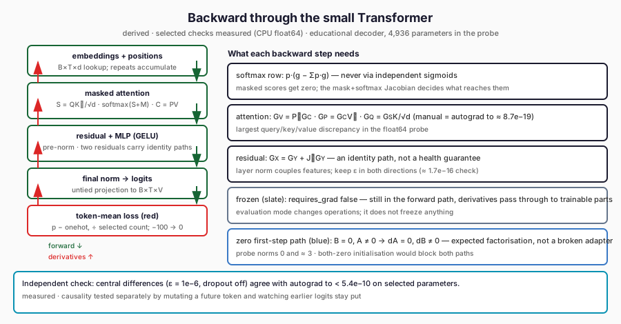
The left column follows the forward chain downward with derivatives returning upward; the right column collects what each backward step needs, including the frozen-parameter and zero-initial-path cases that look like failures but are not. The strip records the independent finite-difference agreement on selected parameters.
Differentiate a linear map and an embedding lookup
For a matrix product $Y=XW$, with upstream derivative $G$, differential notation gives
An embedding lookup is a row selection. Its backward operation adds each selected position’s upstream derivative into the corresponding embedding row. If ID 1 occurs twice, its gradient receives both contributions. Our small independent test sums embeddings for IDs [1, 1, 2]; row 1 receives [2, 2], row 2 receives [1, 1], and unselected rows receive zero. Repeated-token contributions are accumulated, not overwritten.
That example also clarifies why an unused embedding can have a zero gradient while other embeddings train normally. Zero alone is not evidence of a broken backward pass. Ask whether that parameter participated in a scored prediction’s computation.
Pass through softmax and masked attention
For a softmax row $\mathbf p$ and upstream derivative $\mathbf g$, its vector-Jacobian product is
For attention output $\mathbf C=\mathbf P_{\mathrm{attn}}\mathbf V$, the upstream derivative $\mathbf G_C$ gives
A forbidden future score is replaced by a constant before softmax. Its probability is zero and the derivative back through that masked score is zero. This does not require the derivative with respect to the probability tensor itself to be zero: the masking and softmax Jacobian determine which upstream contributions reach the scores.
The forward causality test changes a future input token and verifies that earlier logits remain unchanged. This tests the information restriction directly, independently of a gradient being small. Both checks are useful: an incorrectly broadcast mask may still produce finite gradients while allowing the model to read the answer it should predict.
Residual additions and layer normalisation
For a residual computation $Y=X+F(X)$, the incoming derivative has an identity contribution and a sublayer contribution:
Layer normalisation couples the features within a position. For feature width $d$, define
The stabilising $\epsilon$ remains inside both forward and derivative calculations. Omitting it in one calculation changes the function being checked, especially when the variance is small. A finite-difference disagreement can therefore come from comparing two different normalisation definitions rather than from an autograd failure.
Follow the MLP and the scalar objective
The MLP is a composition of two linear maps and a nonlinearity. For the exact GELU definition used here,
At the output, a single selected cross-entropy term has derivative $p_v-\mathbb{1}[v=y]$ with respect to its logit. Under a token mean, divide that contribution by the total selected-target count. Ignored target positions contribute zero. From there, linear products, normalisation, residual additions and attention carry the derivative backwards.
Our trace retains intermediate gradients for embeddings, queries, keys, values, scores, attention probabilities, aggregated context, residuals and MLP states. A retained intermediate gradient costs memory; it is a teaching instrument rather than the default training configuration. Chapter 11 will measure the different memory categories instead of assuming that the visible parameter arrays describe the whole computation.
Check selected parameters without trusting the backward implementation
For a scalar parameter $w$, a central difference estimates
With $\varepsilon=10^{-6}$, the reference probe observed:
| Selected parameter | Autograd derivative | Central difference | Absolute error |
|---|---|---|---|
| Output weight, ID 79 and feature 0 | 0.02349374836 | 0.02349374828 | $7.9\times10^{-11}$ |
| Query/key/value projection entry 0,0 | -0.003095272024 | -0.003095272039 | $1.5\times10^{-11}$ |
Embedding entry for H, feature 0 |
0.00004130864482 | 0.00004130917830 | $5.4\times10^{-10}$ |
These selected checks are not an exhaustive proof of every derivative. They are an independent way to detect several wrong paths or shape conventions. Very small $\varepsilon$ increases cancellation; a large value measures curvature over too wide an interval. Near a non-differentiable point, the meaning of a numerical check needs further care. Our selected smooth computation avoids that complication.
The bounded CUDA demonstration separately compares FP32 logits and parameter gradients with a CPU model loaded from the same state. It uses absolute tolerance $10^{-5}$ and relative tolerance $10^{-4}$, and the observed comparisons passed. We do not demand binary identity across different devices and kernels, or call a GPU float32 comparison an independent float64 finite-difference check.
Distinguish accumulation, freezing and an initially zero path
Calling backward adds to existing parameter gradients. In a small regression we call it twice on equivalent forward computations and observe twice the first gradient. Clearing gradients with zero_grad(set_to_none=True) then removes that accumulated buffer. An optimiser step does not, by itself, define when those gradients should be cleared.
Freezing a parameter sets its requires_grad flag to false. The model still uses its numerical values in the forward pass. Other trainable weights can receive derivatives through computations containing frozen weights. Our frozen token and position embeddings have no parameter gradient, while the output head still receives a non-zero gradient. Evaluation mode changes operations such as dropout; it does not freeze parameters.
Low-rank initialisation supplies another instructive zero. Write a linear weight as $\mathbf W_0+\mathbf B\mathbf A$, with $W_0$ frozen. If $G$ is the derivative with respect to that effective weight, then
The output of this chapter is a checked derivative path, not an improvement claim. We have tested causality, selected analytical products, central differences, frozen parameters and gradient buffers using one shared model. Chapter 10 now asks how an optimiser turns those gradients into controlled changes to the stored weights.
Further Reading
- Ashish Vaswani et al., “Attention Is All You Need” (2017). Read the source. The architecture paper whose attention, residual and normalisation blocks the chapter differentiates by hand.
- Jimmy Lei Ba, Jamie Ryan Kiros and Geoffrey E. Hinton, “Layer Normalization” (2016). Read the source. The normalisation paper behind the chapter’s lengthiest hand derivation, explaining why the backward pass couples features within a position.
- PyTorch contributors, “Autograd mechanics” (PyTorch 2.6 notes). Read the source. The mechanism reference justifying the warning that autograd records what ran but cannot certify the intended labels or frozen set.