Full, Partial and Parameter-Efficient Fine-Tuning
Choose which parameters may change, count the gradient, optimiser and checkpoint state each choice creates, and compare policies without confusing capacity with merit.
Every fine-tuning run answers a question before the first batch is read: which numbers in the model are allowed to change? Updating everything is the most general answer. Updating only the output layer, only the token embeddings, one Transformer block or a low-rank adapter are narrower answers. Each narrower answer saves something, constrains something and changes what a result can mean.
The usual summary is that parameter-efficient methods are cheaper and full fine-tuning is stronger. That is too vague to act on. Cheaper in which memory term? Stronger at equal learning rate, equal updates, or equal tuning effort? And does a parameter marked trainable actually change during training?
This chapter turns those questions into accounting identities and a controlled experiment. We define a selection policy precisely, derive the gradient, optimiser and checkpoint state it creates, verify those counts against an implementation, and then show why the loss table from the same experiment must not be read as a ranking of methods.
The results below have also been executed in the pinned Docker CPU environment as FT-P5-INTEGRATED-02-25, using the repaired Part IV foundation and local FineTuneLab 0.12.0. The integrated evidence map records source, configuration, environment and artifact hashes for each claim. Earlier staging and authoring comparisons remain historical provenance; they are not independent acceptance. No pretrained-model operation is authorised by these runs.
A selection policy is a set, not a label
Let the model’s parameters be a set of named tensors. A selection policy chooses a subset S of those names. Only tensors in S receive optimiser updates; every other tensor is frozen. The trainable parameter count is
- Full: S contains every parameter.
- Output layer: S contains only the final projection to vocabulary logits.
- Embedding: S contains only the token-embedding matrix.
- Selected block: S contains every parameter of one named Transformer block.
- LoRA: the frozen base gains two factors on one target layer, and S contains only those factors. Chapter 22 derives the layer; we reuse it unchanged.
The original adapter work of Houlsby and colleagues adds task-specific modules while retaining shared frozen parameters; LoRA restricts weight updates through low-rank factors. These are distinct from selecting a subset of existing parameters. BitFit, for example, selects bias terms; that policy is described here as context, not implemented in the five-policy experiment.
Writing the policy as a set has a practical consequence. The name “LoRA” says nothing about which layers carry factors, and “partial fine-tuning” says nothing about which parameters are partial. A result that cannot report S cannot be compared with another result.
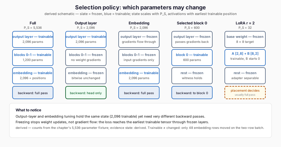
The figure names the five S sets used in the experiment and their trainable counts. Notice that output-layer and embedding tuning hold the same state yet need very different backward passes, and that LoRA’s saving depends on where its factors sit.
Three invariants follow from the definition.
- Membership: the parameters with
requires_grad=Truemust equal S exactly, neither more nor less. - Optimiser membership: the optimiser must own exactly the tensors in S, and its state must contain no tensors belonging to anything else.
- Frozen witness: every parameter outside S must be bitwise unchanged after any number of updates.
Chapter 21 required that after adapter training the optimiser contains only the adapter factors and the base remains unchanged: an adapter-only invariant. That invariant is correct for adapters and wrong for full fine-tuning, where everything is expected to move. A policy system must therefore derive the expected frozen set from the declared method, rather than apply one rule to all methods.
Freezing removes updates, not gradient paths
Freezing a tensor stops its update. It does not stop gradients from flowing through it. Chapter 09 traced the derivative of the loss back through every block; freezing a block removes its weight-gradient accumulation but still requires its input-gradient computation if anything earlier is trainable.
Write the network as a composition of layers, z_(l+1) = f_l(z_l; theta_l), with the loss computed from the final layer. The derivative with respect to a trainable parameter in layer j is
This one observation separates two kinds of saving.
- State saving is proportional to P_S. Gradients, optimiser moments and the checkpointed trainable tensors all shrink when S shrinks.
- Activation saving depends on the position of the earliest trainable parameter, not on P_S. Output-layer tuning needs no backward pass through the blocks. Embedding tuning has a small S in many real models, yet requires the full backward pass because the embedding is the first layer.
LoRA attached deep in the network stops the backward pass at its target only if nothing earlier is trainable and the framework avoids computing unnecessary input gradients. In practice adapters are usually attached in every block, so most of the backward pass still runs. A parameter-efficient method is therefore state-efficient by construction and activation-efficient only by placement.
Derive the state each policy creates
Let P_S be the trainable count, and let FP32 storage use four bytes per element. A gradient buffer exists for every trainable tensor after a backward pass, so
A checkpoint of the trainable tensors stores 4P_S bytes of data plus a header describing names, shapes and offsets. The header grows with the number and length of tensor names, so it is not a fixed percentage.
These formulas say nothing about the frozen weights, which remain in memory for every policy, or about activations, which depend on the backward path above. They are the terms a selection policy actually controls.
Work through the counts on a model small enough to inspect
The experiment uses the book’s explicit causal Transformer from Chapter 09 with vocabulary V = 262, width d = 8, h = 2 heads, MLP width f = 16, context 16 and n = 2 blocks. Its parameter formula, checked in the model constructor, is
The derived state is then:
| Policy | P_S | N_S | Gradient bytes 4P_S | AdamW bytes 8P_S + 4N_S |
|---|---|---|---|---|
| Full | 5,536 | 29 | 22,144 | 44,404 |
| Output layer | 2,096 | 1 | 8,384 | 16,772 |
| Embedding | 2,096 | 1 | 8,384 | 16,772 |
| Selected block 0 | 600 | 12 | 2,400 | 4,848 |
| LoRA, r = 2 | 32 | 2 | 128 | 264 |
The implementation measures these quantities from the live gradient buffers and optimiser state after training rather than computing them from the formula. All ten measured byte counts equal the derived values exactly. The measured checkpoint tensor files were 24,400, 8,464, 8,472, 3,336 and 288 bytes; the differences from 4P_S, from 2,256 bytes for the full policy down to 80 bytes for the output layer, are the safetensors headers.
Notice that the output layer and the embedding have identical trainable counts and identical state, because both are 262 × 8 matrices. Yet their activation requirements differ completely. Output-layer tuning needs gradients only at the final projection; embedding tuning needs the full backward pass. The state table alone cannot distinguish them.
Trainable is not the same as changed
After eight updates the implementation also counts how many elements actually differ from their starting values. The two counts disagree in an instructive way.
| Policy | Trainable elements | Elements that changed |
|---|---|---|
| Full | 5,536 | 3,424 |
| Output layer | 2,096 | 2,096 |
| Embedding | 2,096 | 48 |
| Selected block 0 | 600 | 600 |
| LoRA, r = 2 | 32 | 32 |
The training batch has two rows of nine token positions. Only six distinct token IDs appear at attended positions, so only six of the 262 embedding rows receive a non-zero gradient: 6 × 8 = 48 elements. AdamW with zero weight decay and zero gradient history leaves the other 256 rows exactly unchanged.
The full policy shows the same effect plus one more. Its 3,424 changed elements are 5,536 minus the 2,048 untouched embedding elements, minus 64 untouched position-embedding elements. Positions 9 to 15 never occur, which accounts for seven rows. The eighth unchanged row is position 8. It is occupied in the second sequence, but under the causal shift from Chapter 08 the logit at the final position predicts nothing, and causal attention prevents any earlier position from reading it. Its output never reaches the loss, so its position embedding receives exactly zero gradient.
Neither count is “the” size of the update. Trainable count measures the space the optimiser could explore. Changed count measures what this particular data touched. A policy comparison that reports only the first can overstate how much an embedding-only run altered the model; one that reports only the second can understate how much a different batch could alter it.
The output-layer row shows the opposite case. Softmax cross-entropy sends a gradient to every logit, so every one of the 262 output rows changes even though most tokens never appear as targets. Their logits are pushed down.
Run the controlled comparison
The five policies start from the same seed-37 weights, read the same two-row training batch, use AdamW at learning rate 0.02 with zero weight decay, and take eight full-batch updates in FP32 on one CPU thread. After training, each run saves its trainable tensors, reloads them into a fresh model with the same policy and checks the logits. The maximum reload error was zero for all five. The frozen witness confirmed that no parameter outside S changed in any run.
| Policy | Loss after update 1 | Loss after update 8 | Teacher-forced argmax correct, 5 targets |
|---|---|---|---|
| Full | 4.949223 | 2.473416 | 4/5 |
| Output layer | 5.240241 | 3.810204 | 3/5 |
| Embedding | 5.433372 | 5.326720 | 0/5 |
| Selected block 0 | 5.307708 | 4.563028 | 2/5 |
| LoRA, r = 2 | 5.446692 | 5.410015 | 0/5 |
Before training, every policy predicted 0/5 of the five supervised targets. “Teacher-forced argmax” means the model receives the true preceding tokens and we compare its highest-scoring next token with the label; it is not free generation. All five targets are in the training batch itself.
Why that table is not a ranking
It is tempting to read the table as “full beats output layer beats block beats embedding and LoRA”. The experiment does not support that sentence, for at least four reasons that apply far beyond this toy.
Unequal capacity at equal settings. The policies share a learning rate and an update count, but they do not share an optimisation budget. Full tuning moves 5,536 elements; LoRA moves 32. AdamW normalises each element’s step to roughly the learning rate, so eight steps at 0.02 move LoRA’s few elements only a little. A fair comparison tunes each policy’s learning rate and update count on validation data, which this experiment deliberately does not do.
Initialisation asymmetry. Chapter 22 showed that LoRA’s B factor starts at zero, so the adapter begins as an exact no-op and its first update moves only B. The predictions after eight LoRA updates were identical to the predictions before training. A short run measures this start-up behaviour, not the method’s ceiling.
Training-set evaluation. All five targets are training targets. A higher count means better memorisation of two sequences, which says little about a held-out task. Chapter 06 made the same point from the other direction: a falling training loss does not show that adaptation solved the task.
No uncertainty. One seed and five targets cannot distinguish 3/5 from 2/5 as a property of the method rather than of this initialisation.
What the experiment does establish is narrower and still useful. The five policies are implemented as declared, the membership and frozen-witness invariants hold, the state counts equal their derivations, reload is exact, and the policies produce different learning trajectories from identical starting conditions. Those are the prerequisites for running a fair comparison later.
Design a fair comparison before running one
A comparison between policies needs a stated estimand. “Which policy reaches the best held-out task score when each is tuned within the same compute budget?” is a different question from “which policy reaches the best score at a fixed learning rate?” Chapter 23’s design discipline applies directly:
- Fix the base checkpoint, data splits, tokenisation, loss mask, evaluation contract and seeds across all policies.
- Choose a budget unit and state it: equal updates, equal target tokens, equal wall-clock time or equal peak memory. They give different answers.
- Tune each policy’s learning rate (and, for adapters, rank and scaling) on the validation split only, with the same tuning effort for each.
- Report P_S, changed elements, peak memory and the held-out metric together.
- Keep the protected test split untouched until every selection is complete.
Each row of the table above fails at least two of these requirements, which is why it remains a mechanism check.
When each policy is rational
The derivation suggests when each choice is worth considering, independent of the experiment’s numbers.
- Full tuning is the reference against which others are measured. It has the largest state and the fewest constraints. On hardware where the state fits, it is often the right control even when it is not the final method.
- Output-layer tuning is a linear readout of fixed features. It needs no backward pass through the network and is the cheapest serious baseline. If the base representation already separates the task, it can be sufficient.
- Embedding tuning changes how inputs are represented while every transformation stays fixed. It is useful for new tokens, but for a vocabulary of hundreds of thousands it is not small, and it requires a full backward pass.
- Selected-block tuning concentrates capacity at one depth. Choosing the block is itself a hyperparameter and needs validation evidence.
- LoRA restricts the update to a low-rank subspace per target. Its state is small and its adapter is separable from the base, which matters for storage and composition, but Chapter 22’s caution stands: the rank restriction is an inductive choice, not a guarantee.
Hardware enters as a constraint, not as evidence of quality. If full tuning does not fit, the comparison that matters is between policies that do fit, and the claim must say so.
Failure modes the validator must catch
The implementation’s tests are worth reading as a list of ways a policy can silently lie. Each is a negative test that must raise a named error:
- a parameter outside S marked trainable, or a parameter in S frozen;
- an optimiser that owns an extra tensor or holds state for one it should not;
- an unexpected key or a non-finite value in the optimiser state;
- a frozen parameter that changed, or a frozen witness missing a tensor;
- an adapter checkpoint relabelled as full parameters, or loaded into a model whose starting weights differ from the recorded initial state;
- evidence moved from one run’s configuration to another’s;
- a corrupt tensor file, or an attempt to overwrite an existing checkpoint;
- an adapter whose actual rank or scaling differs from the declared policy.
The third and fifth are the subtle ones. An optimiser built from
model.parameters() rather than the selected list can carry state for frozen
tensors without changing them, inflating memory and making a later unfreeze
behave unexpectedly. A checkpoint without the initial-state identity can be
loaded into a different base and still produce plausible outputs.
What remains unknown
These runs use a random 5,536-parameter model, two training rows and CPU FP32. They establish state accounting and invariant enforcement. They do not establish which policy performs best on any task, how activation memory scales on a real model, or whether the saving in state translates into a saving in peak device memory once activations dominate. No pretrained weights were loaded; real-model comparisons remain blocked by the acquisition gate described in Part IV.
The same experiment was executed twice: once in the engineering staging environment and once in a separate authoring container against the repaired Part IV package. All counts, byte totals, reload errors and predictions matched exactly. Five loss values differed in the seventh significant figure, the expected size of floating-point differences between two builds of the same library.
FineTuneLab
The policies live in the module ftlab.advanced.strategies, integrated with the repaired Part IV package. Selection declares the
policy; apply_selection attaches any adapter and sets membership;
validate_selection checks membership, count and optimiser ownership;
frozen_witness and assert_frozen enforce the frozen invariant; and
save_selected and load_selected write and bind checkpoints to the initial
state, data, configuration and source. The module does not call the Part IV
adapter exporter, and it does not apply the adapter-only rule to full tuning.
The integration candidate is labelled 0.12.0. It is built and tested locally; no package publication or independent acceptance is implied.
Where this leads
Low-rank factors are one way to restrict an update. They add a structured matrix to a frozen weight. The next chapter, Beyond Conventional LoRA, asks what happens when the restriction is placed elsewhere: on activations, on the input sequence, on a weight’s magnitude and direction, or on the rank budget itself. Those methods are not interchangeable, and their differences start in the algebra.
Further Reading
- Edward J. Hu et al., “LoRA: Low-Rank Adaptation of Large Language Models” (2021). Read the source. Freezes pretrained weights and injects trainable rank-decomposition matrices into each Transformer layer, matching full fine-tuning with far fewer trainable parameters. Read it for the rank-deficiency evidence behind low-rank updates.
- Neil Houlsby et al., “Parameter-Efficient Transfer Learning for NLP” (2019). Read the source. Inserts small task-specific modules between frozen layers, reaching close to full fine-tuning on GLUE while adding only a few percent of parameters per task. Read it as the origin of the add-modules family the chapter distinguishes from subset-selection policies.
- Elad Ben-Zaken, Shauli Ravfogel and Yoav Goldberg, “BitFit: Simple Parameter-efficient Fine-tuning for Transformer-based Masked Language-models” (2021). Read the source. Updates only bias terms and matches full fine-tuning on small-to-medium data. Read it as the sparsest selection policy in the literature and as evidence that trainable count alone does not explain adaptation.