Checkpoints, Reproducibility and Recovery
Define exactly what a training checkpoint must contain, distinguish reload, restart, resume and replay, and test exact CPU recovery against deliberate failures without claiming determinism across hardware or library versions.
A training run stops at update 3 of 8. The process was killed, the machine rebooted, or the job hit its time limit. The adapter weights from update 3 are on disk. Can the run continue as if it had never stopped?
Usually the honest answer is “not from the weights alone”. The next update depends on the optimiser’s moment estimates, the learning-rate schedule’s position, the random numbers that will choose dropout masks, the order in which the sampler will deliver examples and how far through that order it has got. Lose any of these and the continued run is a different run that happens to start from the same weights.
This chapter makes that statement exact. It defines a vocabulary that separates several things people call “reproducibility”, derives what a complete training state contains, and then tests a small stochastic CPU run that is interrupted, saved, reloaded and continued. In that one environment, continuation from complete state is bit-for-bit identical to the uninterrupted run. Weights-only continuation is not. Neither result is extended beyond the environment that produced it.
The results below have also been executed in the pinned Docker CPU environment as FT-P5-INTEGRATED-02-30, using the repaired Part IV foundation and local FineTuneLab 0.12.0. The integrated evidence map records source, configuration, environment and artifact hashes for each claim. Earlier staging and authoring comparisons remain historical provenance; they are not independent acceptance. No pretrained-model operation is authorised by these runs.
Name the operations precisely
Six terms are often used interchangeably. They mean different things.
- Reload: load saved weights to evaluate or serve a model. No training continues, so optimiser and sampler state are irrelevant.
- Restart: begin a new training run, typically from the original seed and initial weights. It repeats work already done.
- Resume: continue an interrupted run from a saved state at update k, intending updates k+1, k+2, … to be the ones the original run would have made.
- Exact replay: a resume, or a restart, that produces bitwise-identical state to the uninterrupted run. It can only be claimed for a stated environment.
- Approximate reproducibility: a repeated run that agrees within a declared tolerance or produces statistically indistinguishable results. It is the realistic goal across environments.
- Cross-device reproducibility: agreement between, for example, CPU and GPU, two GPU models, or two library versions. PyTorch’s reproducibility notes state that completely reproducible results are not guaranteed across releases, individual commits or platforms, and need not match between CPU and GPU even with identical seeds.
Chapter 12 resumed a small training loop and recovered its parameters exactly on the same device, and it explicitly declined to promise more. This chapter extends that result with a complete state inventory, a stochastic fixture in which every component matters, and a set of deliberate failures.
PyTorch’s checkpointing tutorial
also distinguishes a general training checkpoint, including optimiser state,
from weights saved for inference. That inventory motivates this exercise; its
exact-resume guarantee comes from the bounded tests below. Python’s
os.fsync documentation
explains the explicit synchronisation call, without supplying a universal
power-loss guarantee for every filesystem.
Training is a state machine
Write one optimiser update as a function
- the model parameters θ_k, both frozen and trainable;
- the optimiser state: first and second moments m_k and v_k for each trainable tensor, and its step count, which enters the bias correction as 1 − β^(k+1) (Chapter 10);
- the scheduler position, which determines η_k;
- the random-number generators that the update consumes: here Python’s, NumPy’s and PyTorch’s CPU generator;
- the sampler state: the current permutation of the dataset, the cursor within it and the epoch;
- the accumulation phase: whether gradients from a partial accumulation are waiting to be applied;
- the loss-scaler state, if dynamic loss scaling is used for reduced precision;
- the step counter and history needed to validate everything else.
If F is a deterministic function in the environment that runs it, then saving S_k completely and restoring it exactly guarantees that every later state matches the uninterrupted run. If any component is missing, the restored S_k differs from the true one, and every later state is computed from a different starting point. The argument is elementary; the work is in making the inventory complete and the restore exact.
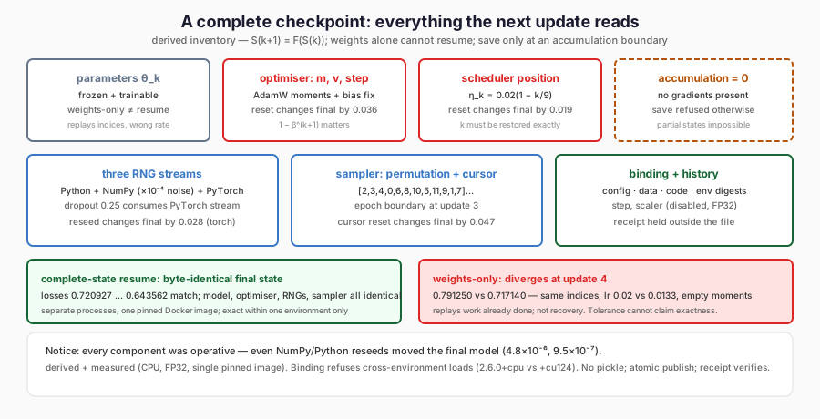
The figure inventories every component the next update reads. Notice that weights alone omit the optimiser, scheduler, generators, sampler and history, which is why weights-only continuation diverges at update 4.
Build a fixture in which every component matters
A test of resumption is only meaningful if the omitted components would change the result. A deterministic, full-batch, constant-rate run would resume exactly from weights alone and teach nothing. The fixture is designed so that each component is operative.
The data are twelve examples. Example i has four binary features, the bits of i, and its label is the exclusive-or of the first two bits. The network is a frozen 4 → 8 linear layer with tanh, dropout at rate 0.25, and a two-class output layer carrying a rank-2 LoRA adapter with α = 2. Only the adapter’s 20 parameters, of 78 in total, are trainable.
Each update draws four examples as two microbatches of two, using accumulation as in Chapter 28. Before each microbatch, the input receives a small perturbation (random.random() + numpy.random.random()) × 10⁻⁴, so both the Python and NumPy generators are consumed. Dropout consumes PyTorch’s generator. The sampler draws a permutation from PyTorch’s generator, walks through it and draws a new permutation at each epoch boundary. The learning rate is η_k = 0.02(1 − k/9), so the scheduler position matters, and AdamW uses weight decay 0.01, so its moments and step count matter.
The run has eight updates. Its first permutation is [2, 3, 4, 0, 6, 8, 10, 5, 11, 9, 1, 7], and the first three updates consume exactly those twelve indices. The checkpoint is taken after update 3, at an epoch boundary: the very next draw will reshuffle using PyTorch’s generator. The fixture therefore exercises the sampler and the RNG in the same moment.
Run the interruption experiment
Four runs share the configuration and seed 37.
- Uninterrupted: eight updates in one process.
- Complete-state resume: three updates, a checkpoint written to disk, a fresh engine that loads it from the file, then five more updates. The fresh engine runs in the same operating-system process. The integrated check additionally saves in process A, waits for it to exit, then loads and continues in process B, comparing against an uninterrupted reference in a third process in the same pinned Docker image.
- Weights-only continuation: a fresh engine whose model weights are copied from the update-3 state, then five more updates.
- Full restart: a fresh engine running all eight updates from the seed.
The recorded per-update losses were:
| Update | Uninterrupted | Complete-state resume | Weights-only |
|---|---|---|---|
| 1 | 0.720927 | 0.720927 | |
| 2 | 0.726608 | 0.726608 | |
| 3 | 0.810076 | 0.810076 | |
| 4 | 0.791250 | 0.791250 | 0.717140 |
| 5 | 0.735644 | 0.735644 | 0.727615 |
| 6 | 0.679898 | 0.679898 | 0.803081 |
| 7 | 0.671109 | 0.671109 | 0.786465 |
| 8 | 0.643562 | 0.643562 | 0.734066 |
The complete-state resume did not merely match losses. Its entire encoded final state, model, optimiser, scheduler, all three generators, sampler and history, was byte-identical to the uninterrupted run’s. That comparison is the real test; equal losses could hide different parameters.
The weights-only run diverged immediately, and the history shows why. Its first update drew indices [2, 3, 4, 0], the same as the uninterrupted run’s first update, because its sampler started again from the seed’s permutation. It also used learning rate 0.02 instead of the scheduled 0.0133, and AdamW started from empty moments. Its final model differed from the uninterrupted one.
The full restart matched the uninterrupted run exactly. That confirms the environment is deterministic, but it is not recovery: it repeated three updates of work. On a long run, restarting is the expensive fallback that a good checkpoint exists to avoid.
Show that each component is operative
The tests prove that a checkpoint missing a component is refused. An authoring probe asked a complementary question: if a component is wrong but the checkpoint is otherwise exact, does it matter? It restored the update-3 state exactly, perturbed one component, ran the remaining five updates and compared the final model with the uninterrupted run.
| Single perturbation after an exact restore | Final model identical? | Largest parameter difference |
|---|---|---|
| None | Yes | 0 |
| PyTorch generator reseeded | No | 0.0280 |
| Sampler cursor reset to zero | No | 0.0473 |
| AdamW moments and step reset | No | 0.0362 |
| Scheduler step counter reset to zero | No | 0.0188 |
| NumPy generator reseeded | No | 4.8 × 10⁻⁶ |
| Python generator reseeded | No | 9.5 × 10⁻⁷ |
Every component changed the result. Two changed it only slightly, because the NumPy and Python generators feed a perturbation of order 10⁻⁴. A tolerance-based check might accept those runs. An exactness claim cannot, because exactness is binary. This is why the definition of “reproducible” must state whether it means bitwise identity or agreement within a tolerance.
The authoring probe exposed a defect in the delivered in-memory interface: training the restored engine modified the original object through aliased optimiser tensors. Integration reproduced that failure before repairing it. The loader now deep-copies the complete validated state before passing any state to PyTorch. Continuing either restored engine leaves the captured state unchanged. The checks compare every nested component, verify independent optimiser tensor storage, exercise in-place moment updates and restore a second engine from the unchanged snapshot. Immediate file encoding had avoided the original alias; the in-memory ownership boundary is now explicit too.
Save only at an accumulation boundary
Gradient accumulation creates a state that is awkward to save: gradients summed over some, but not all, of an update’s microbatches. A checkpoint taken there must store those partial gradients and the phase, or the resumed update will silently omit some microbatches.
The implementation avoids the problem by construction. Saving is permitted only when no parameter holds a gradient, that is, after a complete optimiser update. The checkpoint records the accumulation phase as zero, and the loader refuses any other value. An attempt to save with a gradient buffer present is rejected. The restriction costs nothing in this fixture and makes a whole class of partial states impossible.
The loss scaler is handled the same way. Dynamic loss scaling for FP16 training carries a scale factor and a growth counter that the next update reads. This fixture is FP32, so the checkpoint records the scaler explicitly as disabled with no state, and the loader refuses a checkpoint claiming otherwise. Leaving the field out would make it impossible to tell “no scaler was used” from “the scaler was forgotten”.
Store state safely and publish it atomically
The checkpoint format is JSON with typed values. Tensors are stored as their dtype, shape and base64-encoded bytes; NumPy’s generator state, Python tuples, lists and dictionaries each carry an explicit type tag. There is no pickle, so loading a checkpoint cannot execute code, and the decoder enforces limits on nesting depth, tensor size, element counts and permitted dtypes.
Each checkpoint embeds a binding: the configuration, dataset digest, model identity, adapter method and scaling, the source digest of the training code, the environment (Python, PyTorch and NumPy versions, device and thread count) and the precision. The loader refuses any checkpoint whose binding differs from the receiving engine’s.
Publication follows a fixed sequence:
- Validate the state and refuse it unless the encoded file fits a size limit.
- Create a uniquely named temporary file with exclusive creation, write the
bytes, flush and
fsyncit. - Publish by creating a hard link at the final name. A hard link to an existing name fails, so publication can never overwrite an earlier checkpoint.
- Remove the temporary name.
- Attempt to open and
fsyncthe containing directory after publication and temporary-name removal, recording success or an explicit unconfirmed durability limitation. - Return a receipt: the file’s SHA-256 and length, the envelope digest, the binding digest, the step and digests of the optimiser, RNG, scheduler and sampler components.
Failed publication, including a concurrent publisher or an unsupported hard
link, can leave a fsynced .partial-* file as well as an intentionally
interrupted save. These are retained forensic artifacts, never loadable as
published checkpoints. Inspect and archive a failed run before any deliberate
cleanup; the library does not silently delete its evidence.
    flowchart TD
    A[Validate state and size] --> B[Write temp file, flush, fsync]
    B --> C{Hard link to final name}
    C -- exists --> D[Refuse overwrite, keep evidence]
    C -- created --> E[Remove temp name, fsync directory]
    E --> F[Return receipt, SHA-256 and digests]
    F --> G[Load verifies file against receipt]
    G -- match --> H[Resume: continue as uninterrupted]
    G -- mismatch --> I[Refuse load, engine unchanged]
The diagram follows the publication sequence above. Notice that publication never overwrites and that loading checks the file against a receipt held outside it.
The receipt is retained outside the checkpoint, and loading requires it. Corruption, truncation and substitution are all detected by comparing the file with an independently held expectation, rather than with a digest the file carries about itself.
Atomic visibility, file-content synchronisation and directory-entry
synchronisation are different properties. In the integrated Docker runs, the
file and directory fsync calls both succeeded on the mounted results
filesystem. Where directory synchronisation is unsupported or fails, the
published receipt records UNCONFIRMED; it does not silently promise
directory durability. Hard-link publication still refuses unsupported
filesystems. These tests establish process-level recovery and successful
synchronisation calls, not survival of a real power failure. Filesystem and
device semantics, and newly created ancestor directories, remain limitations.
Inject the failures that matter
The implementation’s tests deliberately break each assumption and check that the load is refused with a specific error, leaving the receiving engine unchanged. The tests construct many of these checkpoints with valid receipts, re-sealed after the change, so they test semantic validation rather than only byte integrity.
| Failure injected | Refusal |
|---|---|
| One byte changed; file truncated | File bytes differ from receipt |
| Published file absent | Checkpoint missing |
| Second save to an existing name | Overwrite refused |
| Save interrupted after writing | Partial file kept under its temporary name; final name never created |
| Unsupported Python object; non-finite JSON number; malformed tensor payload; unknown dtype | Type, value or structure rejected |
| Receipt altered to claim another step | Receipt identity rejected |
| Different dataset, model identity, adapter scaling, source, environment or precision | Binding mismatch |
| Optimiser state absent; moments absent; optimiser owning an unknown parameter | Optimiser state rejected |
| Scheduler position inconsistent with step | Scheduler rejected |
| A generator stream missing or of the wrong type | RNG state rejected |
| Sampler cursor absent, a Boolean, or order not a permutation | Sampler rejected |
| Non-zero accumulation phase; gradients present at save | Accumulation boundary enforced |
| Scaler claimed enabled in an FP32 run | Scaler rejected |
| Step outside the run; history inconsistent with the run | Step or history rejected |
| A frozen base weight changed, container re-sealed | Frozen-parameter change rejected |
| A required top-level field removed | Incomplete state rejected |
| Configuration requesting BF16 | Precision outside the tested profile refused |
The full-parameter mode, in which the whole network trains, also resumes exactly in its own test. All of these tests passed in the engineering staging suite, and the nine Part V test modules (243 tests) passed again in the separate authoring container against the repaired Part IV package.
Same code, different environment
The authoring re-run produced a small, useful demonstration of why the binding
includes the environment. The staging environment reported its PyTorch version
as 2.6.0+cpu; the authoring container reported 2.6.0+cu124, running on CPU.
The checkpoint files therefore differed by exactly one byte in length, 21,237
against 21,238. The version strings differ by two characters; the
complete encoded state differed by one byte. That whole-file difference was
observed, not derived solely from string length. A
checkpoint from one environment would be refused by the other’s loader.
The losses also differed. Six of the recorded per-update losses disagreed between the two environments by at most 6 × 10⁻⁸. Within each environment, the resume was exact; across them, the runs agreed only approximately. Both statements are true, and they are different claims. The book makes the first and does not make the second into a promise.
What this does not establish
The result is narrow by design. It covers CPU, FP32, separate sequential processes with one thread each, checkpoints at update boundaries, and one pinned environment at a time. It says nothing about GPU kernels, which may use nondeterministic algorithms unless configured otherwise, or about dynamic loss scaling in reduced precision. It does not address distributed checkpoints, which Chapter 29 showed add per-rank shards, topology metadata and partial failures. It does not establish equality across library versions or hardware. Receipts establish that a file matches an earlier record, not who produced it or whether its production was authorised.
Part IV’s adapter export and load, in the repaired package, save an adapter for reuse; they do not save a training run for resumption. Confusing the two is the weights-only failure above, made permanent by a file format.
FineTuneLab
The recovery mechanism lives in the module ftlab.advanced.recovery,
integrated in the local 0.12.0 package. Engine holds the complete training state and advances
it; Engine.state, validate_state and restore define, check and apply that
state, validating everything before touching the destination; encode and
decode implement the typed JSON format; save_checkpoint performs atomic,
non-overwriting publication and returns the receipt; read_checkpoint and
load_checkpoint verify the file against the receipt before restoring. The
module is included in the locally verified 0.12.0 wheel, which remains unpublished.
The separate-process evidence compares model and adapter tensors, optimiser,
scheduler, all three RNGs, sampler, step, history, accumulation, scaler and
bindings bitwise. No tolerance is used for that same-environment comparison.
Where Part V leaves us
Part V has asked, in turn, which parameters move, how their movement is parameterised, what objective it serves, how hyperparameters shape it, how it scales across devices, and how it survives interruption. Every chapter has used small models whose every number can be checked, and every chapter has marked the boundary beyond which its evidence stops.
The next part changes the kind of signal the model learns from. Learning From Comparisons Rather Than Demonstrations begins with a different question: what can a model learn when it is told only which of two responses is better?
Further Reading
- PyTorch contributors, “Saving and Loading Models (tutorial)”. Read the source. Distinguishes inference-only state_dict serialisation from general checkpoints carrying optimiser state. Read it as the inventory the chapter’s state machine makes exact; also recommended in Chapter 1 for the reload audit.
- PyTorch contributors, “Reproducibility (notes)”. Read the source. Denies cross-release and cross-platform bitwise guarantees and documents seeding controls. Read it as the official boundary of the chapter’s exact-replay claim; also recommended in Chapters 12 and 19.
- Hugging Face, “Safetensors documentation” (living documentation). Read the source. Defines a tensor format with no executable code and zero-copy loading. Read it as the safe-serialisation counterpart to the chapter’s pickles-free checkpoint.