Deriving the Distillation Objective
The teacher's distribution becomes a training target through KL divergence and a temperature-scaled loss. This chapter derives the objective, checks it against E1, and separates agreement from correctness.
Soften a teacher and a student far enough and the divergence between them almost vanishes. In this chapter’s worked two-class example, the KL divergence between the temperature-scaled teacher and student is \(0.2574\) at \(T=2\) and \(0.0001125\) at \(T=100\). If that number were the training loss, raising the temperature would shrink the teacher’s contribution towards zero. The classical objective multiplies it by \(T^2\), which keeps it between \(1.0296\) and \(1.1250\) at the temperatures the chapter checks. That factor, and the direction in which the divergence is written, are not decoration. They are part of what the student is trained to do.
Chapter 04 ended with a probability distribution. This chapter turns it into a training objective. The teacher supplies a distribution \(p_T\); the student produces a distribution \(p_S\). The student is trained to make its distribution closer to the teacher’s, usually while still learning from the task label. The result is the classical knowledge-distillation objective.
The chapter’s central question is:
Why does matching a temperature-scaled teacher distribution train a student, and how do we know whether that transfer worked?
The answer has two parts. The mathematical part is a divergence between distributions and its gradient. The empirical part is a comparison against a baseline on held-out task data. The first part can be derived; the second cannot be assumed. E1 is the book’s first controlled test, and its result is not the simple success story that the derivation alone might suggest.
The derivation will show that the teacher-matching term can fall while the student’s task accuracy stays the same or becomes worse. That is not a defect in the algebra. It is the difference between matching a distribution and solving a task.
Why the teacher’s distribution is a target
A teacher’s full output distribution contains more than its top-1 label. If the teacher assigns probability \(0.70\) to class A, \(0.25\) to class B, and \(0.05\) to class C, the relative mass says that B is a more plausible alternative than C. A hard label records only that A is correct. Matching the full distribution can therefore give the student a richer signal than matching a single class.
The teacher is not ground truth. Its distribution is a target supplied by a model, and it can be wrong. The objective below treats the teacher as a fixed source of supervision; it does not claim that the teacher is correct. Correctness is measured separately on held-out task data.
KL divergence
For two probability distributions \(p\) and \(q\) over the same finite output space, the Kullback–Leibler divergence from \(p\) to \(q\) is
The divergence is non-negative. One way to see this is to apply Jensen’s inequality to the concave logarithm, summing only over the support \(\{i:p_i>0\}\) with the convention \(0\log(0/q)=0\):
A simple asymmetry check makes the point. Take \(p=(0.9,0.1)\) and \(q=(0.5,0.5)\). Then
Cross-entropy and entropy are related to KL by
A two-class check
Take
The direction of the divergence
The classical distillation objective uses
The direction matters. Reversing it gives
The forward direction, \(D_{\mathrm{KL}}(p_T\parallel p_S)\), penalises a student that assigns near-zero probability to a class the teacher considers plausible. The reverse direction penalises a student that assigns probability to a class the teacher considers unlikely. In a classifier with a fixed teacher distribution, these produce different pressures on the student’s logits. The literature sometimes writes the divergence in the opposite order or calls one direction “reverse KL”; the convention must be read from the equation, not the name.
In the classical objective, the teacher distribution is fixed. The teacher’s parameters are frozen, its logits are detached from the student’s computation, and no gradient flows into the teacher. The student receives the gradient through its own logits. The class or token dimension must align, and the reduction over classes and examples must be stated explicitly.
Deriving the temperature-squared factor
For a single example, let
At \(T=1\), the factor disappears and the gradient is the ordinary \(p_S-p_T\). At large \(T\), the distribution difference is \(O(1/T)\), and the KL gradient carries an additional \(1/T\) from the chain rule, so the unscaled gradient is \(O(1/T^2)\). The \(T^2\) factor compensates for that leading-order suppression. It does not make the gradient exactly independent of temperature for arbitrary logits.
The objective is the classical temperature-scaled form used by Hinton et al. (2015). The chain rule supplies the \(1/T\) factor in the KL gradient. The \(T^2\) multiplier is a chosen compensation for the leading-order temperature scaling; it is not itself a consequence of the chain rule. Together they produce the \(T(p_S^{(T)}-p_T^{(T)})\) gradient.
To see the high-temperature behaviour, write
A numerical check shows the effect. For the two-class example below:
| Temperature | \(D_{\mathrm{KL}}\) | \(T^2D_{\mathrm{KL}}\) | Gradient on first logit |
|---|---|---|---|
| \(T=2\) | \(0.2574\) | \(1.0296\) | \(-0.7070\) |
| \(T=10\) | \(0.0112\) | \(1.1208\) | \(-0.7481\) |
| \(T=100\) | \(0.0001125\) | \(1.1250\) | \(-0.7500\) |
The T=2 entry is the gradient of the scaled KL objective. The \(\lambda=0.5\) mixed soft-term contribution is half of it, \(-0.3535\); the full mixed gradient also includes the hard-label term.
The unscaled KL falls toward zero as the distributions become uniform. The scaled objective approaches a finite limit, and the scaled gradient approaches a finite value. That is the sense in which \(T^2\) compensates.
The expansion uses centered logits because softmax is invariant to a common offset; the offset cancels from the leading term. It assumes fixed finite logits and a fixed number of classes. It does not describe the limit \(T\to0^+\), and it does not claim that the scaled objective is exactly constant at finite temperature. At \(T=1\), the factor is one and the gradient is the ordinary \(p_S-p_T\).
The implementation applies \(T^2\) to a batchmean KL. The per-example
derivation above still describes the gradient of the averaged loss: averaging
over examples commutes with differentiation, and each example contributes the
same \(T(p_S-p_T)\) term before the batch reduction.
The complete mixed objective
The classical objective combines task supervision and teacher supervision:
The hard term teaches the student to predict the task label. The soft term teaches it to match the teacher’s distribution. The coefficient balances the two terms; what it does and does not mean is discussed after the gradient below.
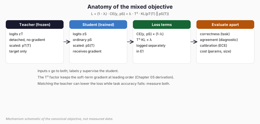
Figure 1. How the pieces combine. The frozen teacher supplies the soft target; the student supplies both distributions; the two weighted terms form the loss; only the student receives gradients. The evaluation on the right stays separate from the training on the left. Mechanism schematic, not measured data.
At \(\lambda=0\), the objective is ordinary supervised training. At \(\lambda=1\), the teacher term is the only supervision in the defined objective. Intermediate values mix the two.
For a single example, with the KL summed over classes, the gradient with respect to the student logits is
The coefficient \(\lambda\) does not mean that the teacher contributes exactly \(\lambda\) of the learning. The hard and soft terms can have different magnitudes, and their gradients can point in different directions. The coefficient is a control on the relative loss scale, and it should be selected on validation data, not on the held-out test set. The endpoints are nevertheless useful checks: \(\lambda=0\) must reduce to the supervised baseline, and \(\lambda=1\) must leave only the teacher term.
In E1, the coefficient is called weight in the arm specification and is set to
\(0.5\) for the mixed arm. The hard term uses the ordinary student logits; the
soft term uses \(T=2\). The two terms are logged separately during training so
their magnitudes can be inspected. A loss weight of \(0.5\) does not mean the
teacher and label each account for half of the learned function; it means the
two loss terms are combined with equal coefficients before their gradients are
summed.
A complete two-class calculation
Use the illustrative setup
Ordinary distributions:
The hard term pushes the first logit up and the second down because the correct class is 0. The soft term does the same here because the teacher, even after softening, assigns more mass to class 0 than the student does. The combined gradient is stronger than either term alone.
The tested distillation_loss implementation returns the same values within
floating-point tolerance. The two-class test in tests/test_losses.py fixes the
values and the gradient. The focused tests also compare the analytic KL gradient
with a central finite difference at double precision.
The example is useful because the student is wrong under the hard label: its ordinary distribution puts \(0.7311\) on class 1, while the label is class 0. The hard term therefore has a large gradient pushing class 0 up. The teacher is right on this example, and the soft term pushes in the same direction, but with a smaller magnitude because the teacher’s softened distribution still gives \(0.2689\) to class 1. If the teacher were wrong, the soft term would pull the student toward the wrong class. The objective does not know which case it is in; the data and the evaluation do.
The mixed loss is not numerically comparable to the hard cross-entropy alone: it includes a second term with a different target and a temperature scale. The useful comparison is between training procedures, not between the raw loss values of different objectives.
The PyTorch mapping
The existing E1 implementation is the authoritative reference. The relevant
functions are in examples/common/losses.py.
kl_divergence(teacher_logits, student_logits, temperature=1.0) computes
teacher_log_probs = F.log_softmax(teacher_logits / temperature, dim=-1)
student_log_probs = F.log_softmax(student_logits / temperature, dim=-1)
return F.kl_div(
    student_log_probs,
    teacher_log_probs,
    log_target=True,
    reduction="batchmean",
)
PyTorch’s F.kl_div(input, target, log_target=True) computes
With input=student_log_probs and target=teacher_log_probs, this is
\(D_{\mathrm{KL}}(p_T\parallel p_S)\), the teacher-first direction. Swapping the
arguments computes the reverse direction, which is a different objective.
reduction="batchmean" sums over classes and divides by the batch size, giving
the mean per-example KL. reduction="sum" would scale with the batch size;
reduction="mean" would divide by the number of classes as well. Changing the
reduction changes the numerical scale and the effective loss weight. The tests
check that batchmean equals the mean of the per-example row sums.
distillation_loss applies the \(T^2\) factor to the raw KL result:
soft = (temperature**2) * kl_divergence(
    teacher_logits,
    student_logits,
    temperature=temperature,
)
total = (1.0 - weight) * hard + weight * soft
The hard term is ordinary cross-entropy on the untempered student logits. The teacher logits are cached and detached; the teacher parameters are frozen. The student receives the gradient.
The code uses log_softmax rather than log(softmax(...)) for numerical
stability. The loss is computed over the class dimension, and the batch
dimension is reduced by batchmean or by the outer loss weighting. The exact
argument order and reduction mode are part of the objective, not implementation
details.
Independent correctness, agreement, and calibration
A distillation run produces three core measurements:
- Teacher quality: the teacher’s accuracy against task ground truth.
- Student quality: the student’s accuracy against independent task ground truth.
- Teacher–student agreement: the fraction of evaluated examples on which the teacher and student predict the same class.
They are not interchangeable. Suppose a teacher is wrong on an example, and the student copies the wrong prediction. Agreement increases, but student accuracy does not. Conversely, a student can disagree with a wrong teacher and be right. The teacher’s quality must be measured on task data, the student’s quality must be measured independently, and the agreement score describes only the relationship between the two prediction sets.
Calibration is a fourth, secondary property: it measures whether predicted confidence matches empirical correctness. E1 reports expected calibration error (ECE) as the weighted mean absolute gap between confidence and accuracy across 15 equal-width confidence bins, using the maximum class probability as confidence. Cross-entropy and calibration error can improve while top-1 accuracy falls, as E1 shows. A lower calibration error is useful evidence about probability quality, but it is not a substitute for task correctness. Müller et al. (2019) show that label smoothing can improve calibration while a teacher trained with label smoothing can be less effective for distillation because its logits lose resemblance information. Calibration and transfer quality are therefore distinct measurements. Chapter 34 develops the measurement framework.
E1: what actually happened
E1 used a self-created four-class spiral, a frozen teacher, a small student, a
hard-label baseline, and a mixed-distillation arm. The primary comparison was
Arm A versus Arm B at \(T=2\) and \(\lambda=0.5\). The test set was held out, the
teacher was trained first, and three seeds were used. The data had 1,200 training
examples, 400 validation examples, and 1,000 test examples. The teacher was
selected by validation cross-entropy; the student arms used their own validation
objectives. The primary record is experiments/E1-classical/manifest.json, group
E1-20261112T233716Z-3bdf03, protocol 1.1; the run source state was commit
165d9a5 with a dirty tree. Full provenance is in planning/05-evidence.md.
    flowchart LR
  T[Frozen teacher] --> E[Held-out test set]
  A[Arm A: hard labels] --> E
  B[Arm B: mixed KD, T=2] --> E
  E --> M[Accuracy, CE, ECE, agreement]
Figure 2. The E1 comparison structure. Both arms share the student architecture, data order, optimiser, and seeds; only the supervision differs. The test set judges all arms once.
| Quantity | Teacher | Arm A: hard labels | Arm B: mixed KD |
|---|---|---|---|
| Parameters | 17,412 | 228 | 228 |
| Artefact size (state-dict bytes) | 69,648 | 912 | 912 |
| Mean held-out accuracy | 99.9% | 66.87% | 64.20% |
| Accuracy SD across 3 seeds | — | 3.62 pp | 1.71 pp |
| Mean cross-entropy | — | 0.8733 | 0.8651 |
| Mean ECE | — | 0.1461 | 0.0894 |
| Mean teacher agreement | — | 66.97% | 64.30% |
Per-seed accuracy deltas (B minus A) are +3.30, -6.10, and -5.20
percentage points; the mean difference is −2.67 percentage points. Full
per-seed values, paired cross-entropy deltas, and the remaining secondary
measures are in experiments/E1-classical/results.md. Mean training time is
5.91 s (A) versus 8.32 s (B) but is host-sensitive and not a capability claim;
peak memory is a cumulative process high-water mark (about 455–458 MB), not a
per-run footprint; latency is diagnostic and host-sensitive. Two of the three
seeds favoured the hard-label baseline; one favoured the mixed student. The
primary directional hypothesis was not supported.
The mixed student had slightly lower cross-entropy and substantially lower ECE. Those are secondary, task-specific observations. They do not establish that calibration improvements outweigh accuracy losses in general, and they do not identify a cause for the accuracy difference. Capacity, teacher confidence, optimisation, the synthetic task, and the bounded hyperparameter search remain plausible explanations. E1 did not isolate them.
The teacher-agreement numbers are close to the accuracy numbers because the teacher was near-perfect on this task. That is a property of E1, not a general law. The teacher was also well calibrated, with a mean ECE of about \(0.006\). A strong, well-calibrated teacher still did not guarantee a more accurate student.
E1 is a controlled comparison on one synthetic task. It is evidence that the
objective did not improve accuracy in this setting; it is not evidence that
distillation generally fails. The negative result is useful because the
hypothesis, baseline, and test set were fixed for the reported protocol 1.1
group. Protocol 1.1 was a documented revision frozen after the first controlled
group, changing instrumentation only; it was in place before the two repeat
groups and is pre-registered only relative to those repeats, not relative to the
first group. It is not a new hypothesis or an independent replication. See
experiments/E1-classical/protocol-corrections.md for the chronology.
The early-stopping limitation
The student arms share the student architecture, initialisation, data order,
optimiser, batch size, maximum epochs, patience, and seed. They do not share the
same validation objective. train_student calls _validation_student_loss with
the arm’s own distillation_loss: Arm A is selected by validation cross-entropy,
while Arm B is selected by the mixed validation objective.
This is a matched-constraints comparison, not a perfectly matched optimisation and model-selection procedure. The difference is a real limitation of the comparison and should be reported alongside the result. It is not a licence to redesign E1 after the fact, and it is not evidence that early stopping caused the accuracy deficit.
A second limit concerns auditability. All 24 primary-group student runs record
epochs_run = 150, the configured maximum, while the teachers stopped at 107,
191, and 147 epochs. The per-run manifests retain the best validation loss and
the epoch count but not the per-epoch histories, which were removed after the run
to keep the evidence compact (see experiments/E1-classical/measurement-notes.md).
The records therefore cannot show whether patience 20 fired or the cap ended
training. No rerun is authorised to recover that diagnostic.
Designing a fair distillation experiment
A defensible experiment starts with a criterion chosen before the result. E1’s criterion was held-out classification accuracy. Other legitimate goals include similar quality with fewer parameters, lower runtime cost, better calibration, specialist performance, capability transfer, or lower cost per correct response. These goals can conflict; a smaller or better-calibrated model is not automatically a better task model.
The design should record the task, data splits, teacher and student identities, access regime, training objective, optimiser, budget, seeds, validation rule, held-out test protocol, metrics, and rights record. The test set must not be used for early stopping, temperature selection, weight selection, or architecture selection. Validation data handles model selection; the test set is used once for the final evaluation.
A matched comparison should also match the model-selection rule. As the early-stopping limitation above records, E1 does not: Arm A is selected by cross-entropy and Arm B by the mixed loss. This does not invalidate the recorded result, but it limits the claim that the two arms differed only in the training objective. The difference is recorded rather than repaired after the fact.
E1 used per-seed synthetic partitions, three seeds, a frozen protocol, and a recorded rights decision. The same partition is shared by all arms within a seed; partitions are regenerated for each seed. Repetition of the same implementation supports reproducibility. It is not independent replication by another implementation or researcher, and it does not establish generality beyond the synthetic task. Three seeds give a weak uncertainty estimate; they do not support a significance claim.
Rights and reproducibility
E1’s data, teacher, and student were created inside the repository. RM-101
covers the action train_and_evaluate_e1; it does not authorise distribution of
the student or unrelated training. The manifest records the source state,
configuration, seeds, and hashes. The rights record is action-specific: a
self-created teacher does not make every future use of the student permitted.
An external teacher’s outputs may be subject to service terms, output-use restrictions, confidentiality, personal-data rules, and training-data permissions. A probability vector is still data. The OpenAI Services Agreement, for example, restricts using outputs to develop competing models (L-016; retrieved 12 November 2026). The legal framework is developed in Chapters 36–39; this chapter uses only the self-created E1 pair.
Limits of this chapter’s evidence
The derivations are established background, and every worked number outside the E1 section is illustrative arithmetic checked against the implementation. The E1 result has the limits recorded beside it:
- Set-up: one self-created synthetic task and one small teacher–student pair.
- Measurements: three seeds, which give a weak uncertainty estimate and do not support a significance claim; training time and latency are host-sensitive diagnostics, and peak memory is a cumulative process high-water mark; none of them is a capability result.
- Implementation: the arms used different validation objectives for early stopping, and the removed per-epoch histories cannot show whether patience or the epoch cap ended student training.
- Scope: repetition of the same implementation is not independent replication, the accuracy deficit has no isolated cause, and the calibration observation does not establish that calibration gains outweigh accuracy losses in general.
What the reader can now build
The reader can now derive and implement the classical objective:
- teacher and student logits;
- temperature-scaled distributions;
- teacher-to-student KL;
- the \(T^2\) scaling and its gradient;
- the mixed hard/soft objective;
- a baseline-matched evaluation with accuracy, cross-entropy, agreement, and calibration reported separately.
The most important lesson is not the formula. It is the separation between matching a teacher and improving a task. A student can reduce its divergence from the teacher while remaining less accurate than the baseline. The derivation tells us what the student is optimised to do; the held-out evaluation tells us what happened. Keeping those two statements separate is the discipline that the rest of the book applies to every distillation method.
What comes next
Part I now has its five chapters: the problem, the taxonomy, the pair, the probability mathematics, and the objective. Part II extends the mechanism to response, logit, feature, relational, sequence, and multi-teacher methods. It begins in Chapter 06 with a question this chapter took for granted: the student matched the teacher’s temperature-scaled probabilities, but it could instead match hard predictions, raw logits, standardised logits, or a decomposition of the target and non-target classes, and each choice preserves different information.
References
Hinton, G., Vinyals, O. and Dean, J. (2015). Distilling the Knowledge in a Neural Network. NIPS 2014 Deep Learning Workshop. arXiv:1503.02531. https://arxiv.org/abs/1503.02531
Müller, R., Kornblith, S. and Hinton, G. (2019). When Does Label Smoothing Help? Advances in Neural Information Processing Systems. arXiv:1906.02629. https://arxiv.org/abs/1906.02629
Legal sources
OpenAI Services Agreement. Updated 1 December 2025; effective 1 January 2026. https://openai.com/policies/services-agreement/ (retrieved 12 November 2026).