Classification, Embeddings, and Retrieval
Can a compact bi-encoder preserve a cross-encoder teacher's ranking behaviour while retaining independently measured retrieval relevance? Contrastive objectives, score distillation, hard negatives, Recall@k, MRR, nDCG, and a bounded E2 study with a weak, seed-concentrated result.
A classifier chooses one label from a fixed set. A retriever ranks a corpus whose size is not fixed, for a query it has never seen. The difference sounds organisational until the teacher arrives: a cross-encoder can read a query and a document together and score the pair, but it must do that for every document at query time. A bi-encoder must turn each side into a vector once, then compare vectors. The compact student is therefore not merely smaller; it is a different kind of function:
Can a compact student preserve a larger teacher’s ranking behaviour while retaining independently measured retrieval relevance?
On our bounded study, the answer is a qualified and uncomfortable “partly”. Adding teacher scores to a contrastive student raised mean nDCG@5 from 0.502 to 0.529, but one seed supplied the entire gain, one seed tied, and one was marginally worse. The teacher-only arm was clearly worse than both. The teacher itself ranked far better than any student (nDCG@5 0.856–0.914), and the best arm’s teacher–student top-1 agreement stayed near 0.27. The student learned some ranking; it did not learn the teacher’s ranking. Those are different claims, and the experiment exists to keep them apart.
Retrieval is ranking, not classification
A retrieval system receives a query \(q\), a corpus \(\mathcal{D}=\{d_1,\ldots,d_N\}\), and a scorer \(s(q,d)\). It returns the documents ordered by \(s\), usually truncated at \(k\). The task’s relevance judgements are a separate object: for each query, a set \(\mathcal{R}_q \subseteq \mathcal{D}\) of documents that actually answer it. In a classified task the label set is fixed and the model chooses one; in retrieval the candidate set is the corpus, and the model chooses an ordering. A classifier’s accuracy is therefore not a retrieval metric, and a retriever’s top-1 score is not its whole ranking.
Our corpus makes the distinction concrete. There are 16 entities and
six relations, giving 96 \((entity, relation)\) pairs. Each pair has
exactly one passage that states the relation for that entity, and one
query that asks for it. A query is the token sequence
[QM, ENT03, WROTE]; its relevant passage begins
[ENT03, WROTE, V18, ...] and continues with five filler tokens. A
passage that begins [ENT03, FOUNDIN, ...] shares the entity but
violates the relation; a passage that begins [ENT07, WROTE, ...]
shares the relation but names the wrong entity. Both are plausible
distractors, and both are non-relevant by construction. Relevance is
a fact recorded when the corpus is generated, not a model’s opinion.
That last sentence carries the chapter’s main discipline. A teacher’s score is evidence about ranking; it is not a relevance label. If the teacher ranks a passage first, the passage is preferred by the teacher, not thereby correct. The evaluation must therefore report two different numbers: task relevance against the construction labels, and agreement between teacher and student rankings. The first can be right while the second is low; the second can be high while the first is wrong.
A classifier is the fixed-label special case. Its scorer produces one logit per class, its softmax is a distribution over a known label set, and its cross-entropy is the same negative log-likelihood as the contrastive objective when the candidate set is the class set. The difference is not the algebra; it is the size and openness of the candidate set, the availability of informative negatives, and the evaluation. A classifier’s label set is closed and its decision is a single label; a retriever’s candidate set is the corpus and its quality is an ordering. The contrastive objective transfers because the algebra is shared; the evaluation does not.
Two architectures, two cost profiles
A cross-encoder computes \(s_\theta(q,d)\) from the pair jointly. It can model token-level interactions between query and document, because both are visible to the same forward pass. The price is architectural: for a corpus of \(N\) documents and a query, a cross-encoder needs \(N\) joint forward passes to rank the corpus. A bi-encoder computes \(u_q=f_\theta(q)\) and \(v_d=g_\phi(d)\) separately, then scores with a cheap similarity such as \(u_q^\top v_d\). Document vectors can be precomputed and indexed, so the query-time cost is one query encode plus a similarity search. The bi-encoder gives up joint token interaction in exchange for an index.
This is the design contrast Reimers and Gurevych make concrete for sentence embeddings (P-071): a cross-encoder is accurate but must score every pair, while a siamese bi-encoder amortises document encoding and compares fixed vectors. Their reported BERT-scale timings are theirs, not ours; the architectural point is what this chapter uses. Izacard and Grave apply the same broad idea to question answering, distilling a reader’s attention signal into a retriever so that query–document labels are not required (P-031). Our teacher is a small cross-encoder scorer rather than a reader, and we do not reproduce either paper’s results.
The parameter counts in our study are modest but the asymmetry is real. The cross-encoder teacher has 2,113 parameters: a shared 64-entry token embedding table of width 16, a 32-unit hidden layer over the concatenated query and document vectors, and a scalar output. The bi-encoder student has 576 parameters: the same vocabulary, width 8, mean pooling, an \(8\times 8\) projection, and L2 normalisation. The parameter ratio is 3.67. That ratio alone does not establish an efficiency gain. The architectural difference does: the teacher’s scoring cost grows with the corpus, while the student’s document encoding is paid once and its query encoding once per query.
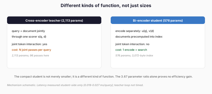
Figure 1. The asymmetry that matters: joint scoring per pair against encode-once plus index search. The 3.67 parameter ratio is arithmetic; the cost structure is the argument. Mechanism schematic.
We measured the student’s query latency, not the teacher’s. At 96 documents, the student’s encode-plus-search step took 0.019–0.027 ms per query across arms and seeds. The teacher would need 96 joint forward passes for the same corpus; we did not time that loop, and we do not invent a number for it. The honest cost claim is therefore conditional: the student has a smaller model, a 3,072-byte document index for 96 eight-dimensional vectors, and a measured tens-of-microseconds query path. Whether that matters at production corpus sizes depends on the index, the hardware, and the candidate-generation stage, none of which this study models.
Embedding geometry
A bi-encoder maps a token sequence to a vector. Mean pooling is the simplest pooling rule: average the token embeddings, ignoring padding, then project. With a projection matrix \(W\) and a pooled vector \(h\), the student produces
The student in this study uses a shared embedding table for queries and documents, mean pooling over non-padding tokens, an \(8\times 8\) linear projection, and L2 normalisation. The teacher uses a separate cross-encoder path: it pools query and document embeddings separately, concatenates them, and passes the pair through a small MLP. The two models do not share a representation space. That matters for what “representation transfer” can mean here. We measure rank transfer through relevance metrics and top-1 agreement; we do not measure representation similarity, because the teacher and student spaces have different dimensions and no alignment map was fitted. A CKA or linear-probe study would answer a different question and was not run.
The contrastive objective
For a query \(q\), let the candidate list be \(C(q)=\{d^+\}\cup N(q)\), where \(d^+\) is a relevant passage and \(N(q)\) is a set of non-relevant candidates. Write the raw similarity \(r_i = u_q^\top v_i\) and the temperature-scaled score \(s_i = r_i/\tau\), where \(\tau>0\) is the contrastive temperature. The InfoNCE loss treats the positive as the correct class in a softmax over the candidate list:
Take a three-candidate illustration with raw scores \(2,1,0\) and \(\tau=1\). The softmax is \((0.6652,0.2447,0.0900)\), so the loss is \(-\log 0.6652=0.4076\). At \(\tau=0.5\) the scaled scores are \(4,2,0\), the softmax is \((0.8668,0.1173,0.0159)\), and the loss falls to \(0.1429\): a lower temperature sharpens the distribution and makes an already-correct positive cheap. At \(\tau=2\) the scaled scores are \(1,0.5,0\), the softmax is \((0.5065,0.3072,0.1863)\), and the loss rises to \(0.6803\): a higher temperature spreads mass to negatives and keeps the gradient alive longer. The temperature is not a quality knob with a universally best value; it sets the scale at which score differences become decisive.
Negative sampling changes the effective training distribution. The softmax denominator contains only the candidates in \(C(q)\), not the whole corpus. In-batch negatives make the denominator cheap but biased by batch composition. Hard negatives, mined by the teacher, put high-scoring non-relevant documents into the denominator, which increases the loss and the gradient on the examples that matter most. Suppose the positive scores 2.0, two hard negatives score 1.5 and 1.0, and an in-batch negative scores 0.5.
With \(\tau=1\), the positive probability is \(0.4551\) and the loss is \(0.7873\). Remove the two hard negatives and keep only the in-batch negative: the positive probability rises to \(0.8176\) and the loss falls to \(0.2014\). The comparison is illustrative, not a controlled measurement—the denominator changed—but it shows the mechanism: harder candidates make the same positive look less certain, and therefore teach more.
Hard negatives also carry a risk. A “negative” that is actually relevant is a false negative; pushing it down teaches the student to reject a correct answer. Our corpus has exactly one relevant passage per query, so the construction labels do not contain false negatives. The teacher’s mined negatives exclude that passage by construction. The teacher’s own training sampler, however, drew random negatives without excluding the relevant passage; we record that defect in the limitations rather than pretending the teacher was cleaner than it was.
Score distillation from a reranker
A cross-encoder teacher does not have to supply hard labels. It can supply a distribution over the candidate list. For the same candidate list, let \(a_T(q,d)\) and \(a_S(q,d)\) be the teacher and student scores, and define
A related objective preserves pairwise similarities between documents rather than query–document scores. That is the relational variant Chapter 09 owns; it was not trained here. The teacher signal in this study is query–document score distillation only, so a reader looking for similarity-preserving representation transfer should treat this chapter as a boundary, not a demonstration.
The crucial limitation is the candidate list. The KL is computed over \(C(q)\), not over the corpus. A student can match the teacher’s local distribution on every training list and still rank the full corpus differently, because the lists are a biased sample of the document space. This is not a technicality; it is the mechanism behind the teacher-only failure below. A local score distribution provides no positive anchor and no global comparison across lists.
Ranking metrics
Three metrics appear in the study, and each answers a different question.
Recall@k asks whether a relevant document appears in the top \(k\). With one relevant document per query, it is 1 if the relevant document is in the top \(k\), and 0 otherwise; the reported value is the mean over queries. It is the bluntest metric and the easiest to interpret.
Mean reciprocal rank (MRR) asks how high the first relevant document appears. For one relevant document at rank \(r\), the reciprocal rank is \(1/r\); MRR is the mean over queries. A relevant document at rank 2 contributes 0.5, at rank 5 contributes 0.2, and absence contributes 0.
Normalised discounted cumulative gain at \(k\) (nDCG@k) asks how much relevance-weighted gain appears in the top \(k\), discounted by position. For binary relevance, with \(rel_i\in\{0,1\}\) at rank \(i=1,\ldots,k\),
With one relevant document per query, \(R@1\) and nDCG@1 are numerically identical, because both are 1 exactly when the relevant document is first. The tables below still report both names where the implementation records both; the duplication is a property of binary relevance, not evidence of two independent measurements.
The frozen E2 retrieval study
The corpus is self-created and fixed: 16 entities \(\times\) 6
relations \(=\) 96 passages, 96 queries, one relevant passage per
query. The corpus fingerprint is
bbc1973817ce79e535d8a90ecbff55110a12a0252d68309b8ab67bc72373c0c8.
Each dataset seed splits the 96 query ids into 64 train, 16 validation
and 16 test queries. Passages for test queries remain in the index:
that is the retrieval task, not leakage. The split is by query id; the
test query ids never appear in a training batch. The per-seed test
split fingerprints are baf0e9ff…, fdc3842b… and 81131473…;
the reconstruction check is recorded in the experiment correction
note.
The teacher is a cross-encoder with width 16, hidden size 32, and 2,113 parameters. It trains for 2,000 updates on 64 query–document pairs per update: eight queries, each with one positive and seven random negatives. Its calibration gate is validation Recall@1 at least 0.40; the measured values were 0.8125, 0.5625 and 0.6875, so the gate passed on all three seeds. The teacher’s held-out test ranking is the ceiling we actually had, not an ideal teacher:
| Seed | Teacher R@1 | Teacher R@5 | Teacher MRR | Teacher nDCG@5 |
|---|---|---|---|---|
| 30 | 0.688 | 1.000 | 0.833 | 0.876 |
| 31 | 0.750 | 0.938 | 0.833 | 0.856 |
| 32 | 0.875 | 0.938 | 0.917 | 0.914 |
The students are bi-encoders with width 8, an 8-dimensional projection, 576 parameters, and L2-normalised outputs. All three arms start from identical initialisations per seed and run exactly 600 optimiser updates with batch size 16 queries, Adam at 0.01, and weight decay 0.0001. The arms differ only in the training signal:
- A-contrastive: InfoNCE with \(\tau=0.07\) on the positive, up to eight teacher-mined hard negatives, and in-batch positives.
- B-teacher: the same contrastive loss plus the teacher score KL with \(T=2\) and weight \(\lambda=0.5\).
- C-teacher-only: the teacher score KL only, with no relevance labels.
The candidate list for each training query is the positive first, then up to eight hard negatives, then in-batch positives up to a cap of 24. The positive-first convention is what the InfoNCE implementation expects. Each arm selects its checkpoint by its own validation objective after the full 600-update budget; the validation objective therefore differs across arms, a comparison limitation we state rather than hide.
What the measurements show
The per-seed held-out results are:
| Seed | Arm | R@1 | R@5 | MRR | nDCG@5 | Agreement@1 |
|---|---|---|---|---|---|---|
| 30 | A-contrastive | 0.312 | 0.625 | 0.462 | 0.474 | 0.250 |
| 30 | B-teacher | 0.375 | 0.750 | 0.511 | 0.556 | 0.312 |
| 30 | C-teacher-only | 0.250 | 0.688 | 0.416 | 0.461 | 0.125 |
| 31 | A-contrastive | 0.375 | 0.750 | 0.519 | 0.563 | 0.312 |
| 31 | B-teacher | 0.375 | 0.750 | 0.523 | 0.563 | 0.312 |
| 31 | C-teacher-only | 0.062 | 0.438 | 0.206 | 0.234 | 0.062 |
| 32 | A-contrastive | 0.188 | 0.750 | 0.399 | 0.470 | 0.188 |
| 32 | B-teacher | 0.188 | 0.750 | 0.397 | 0.468 | 0.188 |
| 32 | C-teacher-only | 0.250 | 0.500 | 0.384 | 0.375 | 0.188 |
The aggregates, with sample standard deviations over three seeds, are:
| Arm | R@1 | MRR | nDCG@5 | Agreement@1 |
|---|---|---|---|---|
| A-contrastive | 0.292 ± 0.095 | 0.460 ± 0.060 | 0.502 ± 0.053 | 0.250 ± 0.062 |
| B-teacher | 0.312 ± 0.108 | 0.477 ± 0.069 | 0.529 ± 0.053 | 0.271 ± 0.072 |
| C-teacher-only | 0.188 ± 0.108 | 0.335 ± 0.113 | 0.357 ± 0.115 | 0.125 ± 0.062 |
These are descriptive three-seed values, not significance tests.
Three observations matter more than the means.
First, the teacher is much better than every student. Its nDCG@5 is 0.856–0.914; the best student mean is 0.529. The student did not preserve the teacher’s ranking. It learned a weak retriever from the same data, with some help from the teacher’s scores.
Second, B’s mean advantage over A is not robust. Per seed, the nDCG@5 difference \(B-A\) is \(+0.082\), \(0.000\) and \(-0.003\). The mean gain is \(+0.027\), entirely carried by seed 30. R@1 is \(+0.0625\), \(0.000\), \(0.000\); R@5 is \(+0.125\), \(0.000\), \(0.000\). The predeclared directional hypothesis—B higher than A on mean nDCG@5—is supported on the mean, but the support is one seed and two ties. This is a weak, seed-concentrated association, not a demonstrated advantage, and it would be dishonest to report only the aggregate.
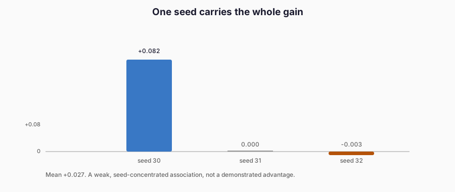
Figure 2. Per-seed B−A nDCG@5: +0.082, 0.000, −0.003. The mean (+0.027) is entirely seed 30. Frozen E2 retrieval measurements.
Third, C is below both A and B on every seed’s nDCG@5, and far below on seed 31 (0.234 against 0.563 and 0.563). Teacher scores alone are a poor training signal for this bi-encoder. The result is not that teacher scores are useless—B’s one gain suggests they can help—but that a score-matching objective without a positive anchor does not teach global relevance.
Teacher–student agreement tells the same story from the other side. B’s top-1 agreement is 0.271 on average, A’s 0.250, C’s 0.125. Low agreement does not prove low relevance: A often disagrees with the teacher and still retrieves the right passage some of the time. High agreement would not prove correctness either. The two numbers must be read together, and neither substitutes for the relevance labels.
Why teacher-only fails
The failure of C is the chapter’s cleanest negative result, and the structure of the objective suggests a mechanical explanation, though the experiment does not isolate it. The KL objective compares the teacher’s softmax and the student’s softmax over the same candidate list. If the teacher puts most mass on the positive and the student learns that shape, the student’s score for the positive rises relative to the hard negatives in that list. But the student never sees the positive against the whole corpus; it sees a sampled candidate list. The global ordering across lists is unconstrained. A student can match every local distribution and still fail to put the positive above the other 95 documents.
On this reading, the positive anchor in A and B supplies the missing global signal. InfoNCE’s target is not “be like the teacher”; it is “put this passage above these candidates.” The teacher’s KL in B adds a softer, list-local preference. The combination gives a small gain on one seed. Without the anchor, on the same reading, C learns a shape without a task.
There is a second reason, specific to this corpus. The candidate list contains up to eight hard negatives and several in-batch positives. The teacher’s scores on those lists may be compressed: a cross-encoder can be confident about the positive while its scores on hard negatives are close together. The KL gradient is \(T(p_S-p_T)\); when the teacher’s distribution is nearly uniform over the negatives, the gradient is small. The contrastive loss, by contrast, always has a positive target and a negative set, so it keeps pushing. This is a hypothesis about the observed failure, not a separately measured decomposition; the experiment did not ablate candidate composition. It is stated as a mechanism worth testing, not as a result.
Cost and efficiency
The measured cost ledger is:
| Quantity | Value |
|---|---|
| Teacher parameters | 2,113 |
| Student parameters | 576 |
| Parameter ratio | 3.67 |
| Student artefact | 2,304 bytes |
| Document index (96 × 8 float32) | 3,072 bytes |
| Student query latency | 0.019–0.027 ms/query |
| Teacher test latency | not measured |
| Teacher training | 3.32–3.47 s per seed |
| Student training | 10.0–15.6 s per arm per seed |
| Teacher forward calls, B/C | 9,984 per seed |
| Total study wall time | 132.1 s |
| Peak process memory | 457.5 MB |
Each of B and C makes 9,984 teacher forward calls per seed: 9,600 training calls (600 updates \(\times\) 16 queries) plus 384 validation calls (24 validations \(\times\) 16 queries). A uses no teacher calls. The teacher’s own training uses 128,000 pair scores per seed (2,000 updates \(\times\) 8 queries \(\times\) 8 pairs). These are operation counts, not prices; no API was used and no provider pricing is invented.
The latency number needs its scope stated. It measures the student’s encode of 16 test queries, the encode of 96 documents, and the similarity matrix, divided by 16 queries. It is not an index build, an ANN search, a batch-throughput measurement, or a production corpus. The 3,072-byte index is a toy. The correct conclusion is architectural: the student has a query-time path that does not scale with corpus size in the way the teacher’s joint scoring does. The incorrect conclusion is that this study demonstrates a production speed-up. It does not.
Rights and provenance
The study uses RM-116, VERIFIED_PERMITTED for
train_retrieval_distillation_e2, reviewed by the author on 16
November 2026 and due for review on 16 May 2027. The corpus, queries,
teacher and student are generated by repository code; no external
corpus, model, API, or paid inference is used. Relevance labels are
construction facts. The embeddings and cached teacher scores are
derived artefacts of that corpus, and the rights record forbids
redistribution beyond the study artefacts. No personal data is
present.
A retrieval corpus is not automatically free to use just because it is downloadable. A compiled database can attract a sui generis right under Directive 96/9/EC for substantial investment in obtaining, verifying, or presenting its contents (L-026). This chapter’s corpus is synthesised, so no third-party database is extracted; the record still exists because the next corpus may not be synthetic. The legal finding is dated and action-specific; it is not legal advice, and it does not resolve the rights of a future corpus.
Limitations
The study is one synthetic corpus, three seeds, tiny models, and a single relevant passage per query. Binary relevance makes nDCG@1 and R@1 identical and removes graded-relevance questions. The contrastive temperature (0.07), KL weight (0.5), KL temperature (2.0) and hard-negative depth (8) are single fixed values; no sweep was run. The teacher’s random-negative sampler did not exclude the relevant passage, so some teacher training pairs were contradictory; the teacher’s measured test ranking is the quality actually obtained, and the effect of that label noise on B and C is not measured.
Validation candidate lists omit in-batch negatives, unlike training lists, so each arm’s checkpoint selection distribution differs from its training distribution. The teacher’s latency was not measured. No out-of- distribution query set was evaluated; the held-out split is a query split, not a distribution shift. No representation-similarity or linear-probe analysis was run, so “representation transfer” is not measured. No external replication and no independent review exist.
Three record-level defects are also disclosed rather than buried.
RESULTS.md prints the training-query count (64) under an N-q
column while the metrics use 16 held-out test queries; the chapter
reports 16. The runner mined hard negatives from train and validation
queries, not train only as the protocol sentence says; test queries
never entered training, and the separately computed test hard-negative
list was unused. The protocol names a superseded run that is not
present in the repository; the cited run’s manifest and source hashes
are intact. These are reporting and preservation defects, not changes
to the measured values. They are recorded in
experiments/E2-retrieval/results-correction-1.md and
planning/00-dfp-11-run-history-gap.md.
Chapter 08 owns feature alignment and Chapter 17 owns the instruction-model baseline whose fixed-update discipline this study follows; this chapter applies those ideas to a retrieval scorer without re-teaching them. Chapter 29 extends the question to multimodal embeddings, Chapter 34 owns ranking evaluation, and Chapter 37 owns corpus copyright.
What comes next
The chapter opened with the difference between choosing a label and ranking a corpus. It closes with the difference between matching a teacher and retaining a task. The student’s relevance improved only weakly, and only on one seed; the teacher’s ranking was not transferred; the teacher-only arm failed. The next chapter changes the output object again. Code generation must produce a structured artefact that compiles or executes, so correctness is not a ranking over candidates but a property of the generated program. Chapter 25 asks what supervision, validation, and evaluation look like when the student’s output must run.
References
Izacard, G. and Grave, E. (2021). Distilling Knowledge from Reader to Retriever for Question Answering. International Conference on Learning Representations (ICLR). arXiv:2012.04584. https://arxiv.org/abs/2012.04584
Reimers, N. and Gurevych, I. (2019). Sentence-BERT: Sentence Embeddings using Siamese BERT-Networks. Proceedings of EMNLP 2019. arXiv:1908.10084. https://arxiv.org/abs/1908.10084
Legal sources
Directive 96/9/EC of the European Parliament and of the Council of 11 March 1996 on the legal protection of databases. In force 27 March 1996. https://eur-lex.europa.eu/eli/dir/96/9/oj (retrieved 12 November 2026). Cited as L-026 for the sui generis database-right context; not legal advice.