Data Filtering and Curriculum Learning
Filtering decides which examples remain; curriculum decides the order they are presented. This chapter separates the two interventions, derives their effect on the training distribution, and tests them in a controlled E3 ablation with real student training.
Chapter 14 generated 2,304 candidates and measured what generation produces. This chapter asks what to do with them: which examples the student should see, in what order, and what the selection rule silently optimises. The central argument is:
Filtering and curriculum learning are interventions on the teaching distribution. They can remove noise, improve training efficiency, and change learning dynamics — but they can also remove useful diversity, overrepresent easy examples, and cause systematic failures on underrepresented cases.
The chapter ends with a controlled experiment that trains real students under four regimes. The regimes shared their nominal settings but not their actual training: the curriculum arms ran fewer optimiser updates than the random-order arms. Its headline result is negative, and it is reported exactly as found: on this task, neither filtering nor curriculum ordering improved the student. A smaller, cleaner, better-ordered dataset produced worse students, not better ones — and understanding why is worth more than a positive result would have been.
Not all teaching examples are equally useful
The Chapter 14 pools contain three kinds of rows: oracle-correct examples, exact duplicates of earlier rows, and a small number of well-formed but wrong outputs from the scripted teacher (7–10 per seed, roughly 1%). The duplicates teach nothing new. The wrong outputs teach something false. The temptation is to remove both and train on what remains — and the temptation conceals two questions. First, does removal actually help the student, or does it merely make the dataset statistics prettier?
Second, what else does the removal rule take out alongside its intended target? A deduplication rule, for instance, disproportionately removes short examples on this task (retention 0.68 for length 4 versus 0.94+ for lengths 6–8), because collisions concentrate in the smallest subspaces. Nothing about “remove duplicates” announces that it is also, quietly, a length filter. Every selection rule has a shadow: the part of its behaviour the rule’s name does not describe. This chapter is about measuring shadows.
KD-021 and curriculum learning
Curriculum learning (KD-021) is the arrangement or weighting of training examples according to an explicit schedule — often by difficulty, but also by diversity or other learning-relevant properties. The registry definition is deliberately behavioural: a curriculum is a training strategy, not a quality score. A filter that keeps “good” examples and a schedule that presents easy examples first are different objects that act at different times (before training versus during training), and the experiment in this chapter controls them independently precisely so their effects — and their interaction — can be told apart.
The standard vocabulary, following Bengio et al. (2009): easy-to-hard presents low-difficulty examples first and adds harder ones over time; hard-to-easy reverses the order; random order is the baseline every schedule must beat; mixed curricula interleave the two ends. Difficulty-weighted sampling generalises fixed orders by sampling each example with probability proportional to a time-varying weight. Diversity-aware ordering spreads coverage deliberately rather than hoping shuffling provides it. None of these is universally optimal — the original curriculum paper frames its method as a continuation heuristic for non-convex optimisation, reports gains in its own settings, and fixes its pace arbitrarily. A curriculum is a bet about optimisation dynamics, not a theorem about learning.
Filtering versus ordering
Filtering determines which examples remain. Curriculum determines how the survivors are scheduled or weighted during training. The two compose — the Chapter 15 ablation has a both-interventions arm — but they must not be confused, because they fail differently. A filter’s failure is subtractive: support lost, coverage narrowed, rare cases deleted. A curriculum’s failure is temporal: the student converges before the hard examples arrive, or sees easy examples so often that capacity is spent on what it already knows.
The pilot run for this chapter demonstrated the second failure concretely: validation-based early stopping fired during the easy-only phase and the schedule never reached harder examples at all. The protocol was amended so stopping is deferred until the final phase — and the amendment is recorded here rather than hidden, because the interaction between stopping rules and schedules is itself a finding: a curriculum evaluated under a stopping rule that cannot see it through is not an evaluation of the curriculum.
How selection changes a distribution
Let the candidate distribution be \(P_G(x,y)\), as in Chapter 14, and let a selection rule be \(a(x,y)\in[0,1]\). The selected distribution is:
\[ \frac{P_G(x,y)a(x,y)}{Z}, \qquad Z = \mathbb{E}_{P_G}[a(x,y)], \]
where the normaliser \(Z\) is the retention rate — the fraction of candidates the rule keeps. This is the same mathematics as Chapter 14’s rejection sampling, applied one stage later: generation filtered the generator’s output, and now selection filters the candidate pool. The consequence is identical in form and different in meaning. A filter that keeps 90% of examples (\(Z=0.9\)) barely moves the distribution; one that keeps 10% replaces it. And crucially, \(a(x,y)\) is never uniform in practice: a confidence filter keeps examples the teacher already finds easy, a length filter keeps short sequences, a diversity filter keeps outliers. Each filter embodies assumptions about which examples are valuable, and the retention rate per group —
\[ r_g = \frac{N_{\mathrm{retained},g}}{N_{\mathrm{candidate},g}} \]
for any group \(g\) with nonzero denominator — makes those assumptions visible. The audit in this chapter reports \(r_g\) by length band, generator mode, and template family for the actual filter, and the numbers show the shadow described above: dedup retention of 0.68–0.73 on length-4 inputs against 0.90+ elsewhere.
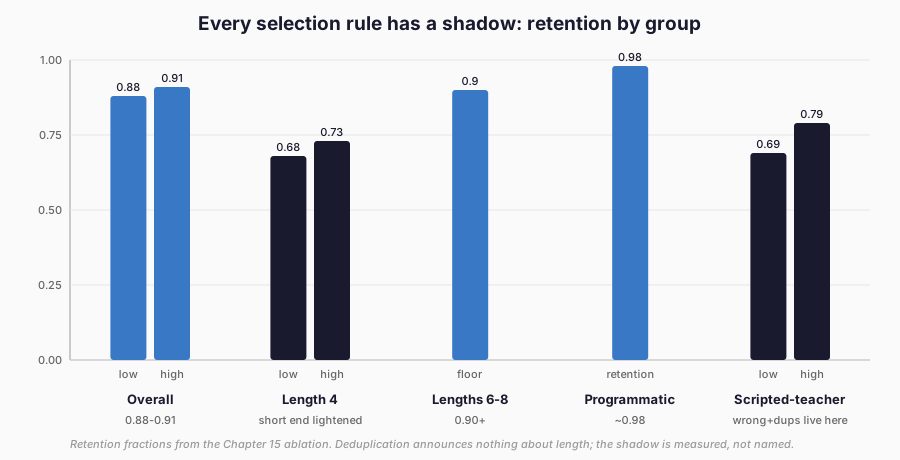
Figure 1. Retention by group for the ablation filter. The aggregate (0.88–0.91) hides the short-end lightening and the mode skew. Chapter 15 measurements.
Quality and confidence filtering
A quality filter keeps examples that pass some bar: structural validity, oracle correctness, teacher confidence above a threshold, length within bounds, or novelty against the retained set. The ablation’s filter uses the first two plus deduplication: recompute the oracle transform and keep exact matches (removing the 7–10 wrong outputs per seed), then keep the first occurrence of each exact input/output pair (removing 50–68 duplicates per seed). Threshold source: the task oracle and the identity definition — train/val evidence only, never test outcomes.
Confidence filtering deserves a worked example because it is the most popular and the most misunderstood. Suppose five candidates carry teacher scores 0.9, 0.7, 0.7, 0.4, and unknown (the teacher declined or the value is non-finite). A threshold of 0.7 keeps the first three and rejects the rest — with two distinct rejection reasons: below-threshold versus unknown-confidence. The distinction matters. Below-threshold is a judgement; unknown-confidence is missing data, and treating missing scores as zero silently converts “the teacher did not answer” into “the teacher is certain this is bad”.
Our implementation rejects non-finite and missing scores with explicit reasons and never invents a score: a filter that hallucinates its own inputs is not a quality control. And the deeper caveat stands regardless of implementation: confidence need not equal correctness. A teacher is most confident exactly where its biases are strongest, so a confidence filter preferentially retains the teacher’s comfort zone — which is why the ablation deliberately uses oracle correctness instead of confidence, and why confidence appears here as a fixture, not a measurement.
Correctness verification
The oracle is the verifier in this study: the deterministic reverse-complement transform from Chapter 13 decides correctness independently of any teacher. That independence is the point. A verifier scores outputs against the task; a teacher generates them. Using the teacher’s own confidence to filter the teacher’s own outputs is circular in a way that using the oracle is not — though it has its own limit: verification certifies the answer, not the reasoning, and a verifier that is wrong (or partial, covering only checkable properties) becomes a second teacher with unexamined authority.
Here the oracle is total over the input space, so the limit does not bind; the chapter states the general warning anyway, because most real tasks have no total oracle, and filtering by an imperfect verifier is then filtering by an imperfect teacher under a better name.
Diversity filtering
Diversity selection keeps examples that add coverage: deduplication, near-duplicate capping, stratified sampling, or clustering. The ablation’s exact-dedup step is the minimal version — first occurrence kept, re-emissions counted (50–68 per seed, concentrated, as noted, on short inputs). Near-duplicate pairs are reported at the Chapter 14 Jaccard threshold (0.9) but not filtered in the main arms: on this tiny space the threshold flags thousands of pairs per pool, and filtering on it would delete most of the data.
That restraint is itself a decision the audit records. Diversity filtering has a failure mode worth naming: optimising diversity without measuring task relevance keeps exotic examples at the expense of representative ones. A pool with one example of everything and mastery of nothing is diverse and useless. Coverage of known task categories (lengths 4–8, all four symbols, all template families) is necessary; coverage of the underlying task distribution is the actual goal, and the two are not the same.
Difficulty measurement
Candidate difficulty in this study is \(d = \mathrm{len}(\mathrm{input}) + 0.5\times(\mathrm{max\_repeat\_run} - 1)\): input length plus half a point per extra repeated adjacent symbol. Both components come from the Chapter 13 E3 difficulty rubrics — output length (errors compound per token) and repeated-symbol runs (local regularity).
The score is a complexity proxy and is explicitly NOT validated as empirical student difficulty: nothing in this book shows that a length-8 example is harder for the GRU student than a length-4 one, and the chapter refuses to smuggle that claim in through the notation. Every use of \(d\) below is labelled a proxy. Ties are broken by a seeded random key, so equal-difficulty examples have a deterministic but arbitrary order — documented in the curriculum manifest, reproducible from the seed.
Easy-to-hard and alternative curricula
Let \(d_i\) be example \(i\)’s difficulty and \(t\) the training phase. A time-varying weight \(w_i(t) = g(d_i, t)\) yields the sampling probability:
\[ P_t(i) = \frac{w_i(t)}{\sum_j w_j(t)}, \]
for non-negative weights with a positive denominator. The ablation’s easy-to-hard schedule is the simplest cumulative version: sort by \((d_i, \mathrm{seeded\_tiebreak})\), split into three chunks, and make weights uniform over the available prefix (phase 0: easiest third; phase 1: easiest two-thirds; phase 2: all). Each phase’s weights normalise to 1 by construction — asserted in code, not assumed. Random order ignores difficulties entirely (one seeded shuffle, then per-epoch reshuffles). Hard-to-easy and mixed (interleaved ends) schedules are implemented and tested but not run as arms: the ablation budget covers four arms, and the contract’s required comparison is filter × easy-to-hard.
The cost of removing difficult examples
Every filter removes something it did not intend. The fixture demonstration makes the mechanism unmistakable: take eleven candidates, ten of length 4–6 and one of length 8, and apply a length filter that keeps inputs of length at most 6. Correct-label rate rises (if the long example happened to be wrong), duplicate rate falls, the report looks better — and length-8 coverage goes from present to absent. Retention for the length-8 group is 0.0: support lost. The filter did exactly what it was told; what it was told was the problem.
The real filter shows the milder, honest version of the same effect. Overall retention is 0.88–0.91 — a flattering aggregate. By length band it is 0.68–0.73 for length 4 against 0.90+ for lengths 6–8. By generator mode it is ~0.98 for programmatic examples against ~0.69–0.79 for scripted-teacher examples (where the wrong outputs and duplicates live, as designed). No group is deleted entirely — support loss is none — but the composition shift is real and directional: the filter lightens the short end and the scripted-teacher mode.
A downstream analyst who notices “the student rarely sees length-4 inputs” would be looking at a filtering artefact, not a task property. The E3 data contains no protected-group information and no demographic attribute is invented; the demonstration uses task categories (length bands), which is where the actual bias in this study lives.
The frozen E3 ablation
Four arms on one shared eligible population per dataset seed (0, 1, 2):
| Arm | Filtering | Curriculum |
|---|---|---|
| A | none (raw eligible) | random order |
| B | oracle-correctness + exact-dedup | random order |
| C | none (raw eligible) | easy-to-hard, 3 cumulative phases |
| D | same filter as B | easy-to-hard, 3 cumulative phases |
The eligible population is the Chapter 14 frozen run’s 768 candidates per seed minus 22–35 structurally invalid rows (bad tokens, truncated outputs — untrainable under the output contract) minus 91–111 rows whose inputs collide with the regenerated validation or test splits (contamination guard). The guard matters: about 12–14% of candidates share inputs with the held-out partitions, concentrated on short lengths where the 87,296-strong space is densest. Structurally valid but wrong outputs (7–10 per seed) stay in the raw arms and are removed only by the declared filter — the quality effect is never hidden inside baseline preprocessing.
The student is the E3 precursor architecture (GRU encoder-decoder, vocab 7, embed 8, hidden 24, ~5,127 parameters) with the precursor optimiser (Adam, lr 0.003, weight decay 0.0001, batch 64, up to 60 epochs, patience 10 on validation oracle NLL). Same initialisation across arms within a seed. Random arms stop from epoch 1; curriculum arms defer stopping until the final phase so the schedule runs its course.
Nominal settings were shared (same epochs, batch, optimiser,
initialisation, checkpoint rule), but actual optimiser updates and token
exposures were NOT matched: random arms ran 600–660 updates, curriculum
arms 360–440. Steps, tokens, and
unique-example exposures are measured per arm and reported alongside
correctness, and the package comparison below must be read with that
mismatch in view. Rights: RM-107 (train_and_evaluate_e3_filter_curriculum,
verified-permitted), gate passed before training. No external data,
models, APIs, or paid inference.
Two discarded pilots preceded the frozen run and are disclosed, not buried: a 30-epoch budget that stopped all arms before learning took off (amended to 60 before any valid run), and a padding-length mismatch (length-12 training rows against length-10 bundle rows) that stalled every arm at floor. Both were implementation defects found before any arm comparison existed to tune against; the design — arms, filter, schedule, seeds, thresholds — never changed.
Measured student results
The frozen run (E15-20261115T160137Z-55eb1e) trained 12 students (4
arms × 3 seeds). Held-out greedy exact match against the oracle:
| Seed | A (raw/rand) | B (filt/rand) | C (raw/curr) | D (filt/curr) |
|---|---|---|---|---|
| 0 | 0.365 | 0.296 | 0.055 | 0.044 |
| 1 | 0.639 | 0.595 | 0.387 | 0.242 |
| 2 | 0.245 | 0.100 | 0.028 | 0.019 |
Aggregates (mean ± SD over 3 seeds): A 0.416 ± 0.202, B 0.330 ± 0.249, C 0.157 ± 0.200, D 0.102 ± 0.122. Token accuracy follows the same ordering (A 0.878, B 0.842, C 0.738, D 0.705); invalid-output rate is 0.000 in every arm — when the student is wrong, it is wrong fluently. Seed spread dominates everything: seed 1 learns well in every arm, seed 2 poorly, and the per-seed ordering is consistent (filtering and curriculum both hurt on every seed, and the combined arm D is lowest on every seed).
The answer to the chapter’s question is therefore negative in both parts. Filtering removed ~9–12% of rows (wrong outputs plus duplicates) and produced worse students on all three seeds. Curriculum ordering produced substantially worse students than random order in the same data. The combined arm is worst of all. Nothing here is a significance test (three seeds cannot carry one), and no causal decomposition is claimed: the filtered arms also trained on fewer examples with fewer updates (540–600 versus 600–660), and the curriculum arms saw harder examples less often by construction.
The experiment supports a package comparison — these interventions, as implemented, did not help — and that is all it supports. A negative result with a controlled design is evidence; a negative result presented as proof that filtering never works would be the same volume-equals-value confusion from Chapter 14 in reverse.
Why might cleaner data teach worse? Three candidate mechanisms, stated as hypotheses, not findings: duplicates act as implicit upweighting of common patterns, and removing them flattens useful frequency signal; the wrong outputs are too few (~1%) to matter, so the filter’s main effect is data loss, not noise removal; and the phased curriculum spends the early budget where validation is uninformative, then under-trains the full distribution (curriculum arms ran 360–440 updates versus 600–660 for random arms). Each is testable in a follow-up; none is claimed here.
Coverage and selection bias
The selection audit (per seed, in selection-audit.json) reconciles
exactly: source 768 = excluded-structural (22–35) + excluded-overlap
(91–111) + eligible (622–655); eligible = filtered (546–589) + removed
(57–76: 7–10 oracle-mismatch, 50–68 exact-duplicates). Fingerprints for
the eligible and filtered populations are recorded. Retention by length
(0.68–0.73 at length 4, 0.90+ at 6–8) and by mode (~0.98 programmatic,
~0.69–0.79 scripted-teacher) quantifies the shadow: per seed 0, the
filter kept 221 of 223 programmatic rows but only 161 of 204
scripted-teacher rows, and length-4 rows were removed far more often than
length-8 rows (27% versus 3–7% removed).
Template families within mode B retain evenly — the phrasing templates carry no quality signal, as designed. Coverage before and after: all length bands and all modes survive (support loss: none), all entropies near 2.0 bits, provenance complete for kept and rejected rows alike — rejected candidates keep their records with reasons, never silently dropped.
Training efficiency and learning curves
Filtering shrinks the dataset and therefore the per-epoch update count; curriculum phasing shrinks it further in early phases. Measured totals: A 600–660 updates, B 540–600, C 420–440, D 360–420; tokens and unique exposures scale accordingly (A sees ~270–283k tokens over 646–655 unique examples; D sees ~150–160k tokens over 546–589 uniques — roughly 60% of the random arms’ exposure).
The curriculum arms’ early phases train on ~200 examples per epoch and validate on the full difficulty range — validation barely improves until the final phase, and without the final-phase stopping deferral they would have stopped before seeing hard examples at all. That interaction is the dynamics finding of this chapter: a schedule and a stopping rule are a joint system, and evaluating one under a rule calibrated for the other measures the mismatch, not the method. Per-accepted-example cost is CPU wall time (whole study under ten minutes for 12 students); no provider pricing exists and none is invented.
Rights and provenance
RM-107 covers exactly this ablation’s action; the gate passed before training, and a wrong action is refused (tested). Filtering decisions are provenance: every kept and rejected row links its candidate id to the filter id, version, configuration, and reason. Removing examples does not remove obligations — derived data inherits its sources’ terms, and the study’s no-redistribution condition reflects that. RM-104’s pending re-attestation remains open and untouched; nothing here trains under it or extends it. Personal data and subgroup impacts: the E3 data is symbol strings with no personal content and no protected-group information; the bias measured is by task category, and the record says so instead of inventing demographic coverage it does not have.
When filtering or curriculum fails
Our negative result joins qualified literature, not slogans. Bengio et al. (2009) introduce curricula as a continuation-method heuristic with arbitrarily fixed pacing — useful, not universal. Xie et al. (2023, DoReMi) optimise domain-mixture weights with a small proxy model and Group DRO, then resample: it is mixture optimisation for pretraining, not per-example easy-to-hard, and the chapter does not conflate the two; their 2.6× step savings and +6.5-point few-shot gains are paper-specific and not replicated here.
Chen et al. (2023, AlpaGasus) filter 52k Alpaca examples to 9k with ChatGPT quality scores and report better instruction-following with faster training — a genuine filter-smaller-beats-full result, but one whose judge (LLM scores) and evaluations (GPT-4, human) are paper-specific and not reproduced here. The pattern across all three: selection helps when the filter removes what the student cannot use and keeps what it must learn — and the only way to know is a controlled comparison like this chapter’s, reported whether it succeeds or not.
Limits of this chapter’s evidence
- Set-up: one synthetic sequence task with a tiny string space and a small GRU student. Difficulty is an unvalidated complexity proxy.
- Measurements: three seeds, and the seed spread dominates the differences between arms. Nothing here is a significance test.
- Implementation: the arms shared nominal settings, not actual training. Optimiser updates ran from 600–660 for the random-order raw arm down to 360–420 for the filtered curriculum arm, so the arms are not budget-matched. Three pilots preceded the single reported run and are disclosed above.
- Scope: the result compares intervention packages; it does not separate the effect of fewer updates from the effect of the selection or ordering. The three mechanisms offered for the negative result are untested hypotheses, and the DoReMi and AlpaGasus results are their authors’ and were not replicated.
Preparing for dataset distillation
Filtering subtracts examples; curriculum reorders them. The next compression step is stronger: synthesise a small dataset that trains a student to approximate one trained on the full data — dataset distillation, Chapter 16’s subject. It starts from this chapter’s outputs: the eligible population with fingerprints, the audit that says what was removed and why, the curriculum code with its schedule manifests, and a caution the ablation earned — that a smaller dataset is a hypothesis about what matters, and hypotheses need held-out evidence.
The gradient-matching and trajectory-matching methods of Chapter 16 optimise the dataset itself rather than selecting from it; they inherit every selection-bias question raised here, with higher compute bills attached. The reader who can answer “what did this rule silently optimise?” for a filter is ready to ask the same question of a synthesiser.
References
Bengio, Y., Louradour, J., Collobert, R. and Weston, J. (2009). Curriculum Learning. Proceedings of the 26th Annual International Conference on Machine Learning, pp. 41–48. https://doi.org/10.1145/1553374.1553380
Xie, S. M., Pham, H., Dong, X., Du, N., Liu, H., Lu, Y., Liang, P., Le, Q. V., Ma, T. and Yu, A. W. (2023). DoReMi: Optimizing Data Mixtures Speeds Up Language Model Pretraining. Advances in Neural Information Processing Systems 36. https://arxiv.org/abs/2305.10429
Chen, L., Li, S., Yan, J., Wang, H., Gunaratna, K., Yadav, V., Tang, Z., et al. (2024). AlpaGasus: Training A Better Alpaca with Fewer Data. arXiv:2307.08701. https://arxiv.org/abs/2307.08701