Choosing the Right Student
How do we choose a student when correctness, latency, memory, and cost compete? A one-host inference benchmark, per-family Pareto analyses, and a constrained-selection rule that picks the calibrated student over the accurate one.
Every experiment so far asked whether the student learned. This chapter asks whether the student is worth deploying — a different question with a different kind of answer. Learning is measured against ground truth; deployment is measured against constraints. A model that scores highest and misses its latency budget by a factor of ten is not the best student. It is a failed deployment:
Which student is the right engineering choice for a stated task, budget, and deployment environment?
The honest answer this chapter defends is that there is no such thing as the right student, only the right student for stated constraints — and that distillation, as practised in this book, never changes what a student costs to run.
In E1–E3 every distillation arm trains the same architecture as its baseline, so all arms in a family share one deployment profile and differ only in correctness. E4 is the one exception, and not because of distillation: its answer-only baseline is a smaller policy than the two trajectory arms, which share one architecture. The choice of architecture is made before distillation starts; distillation moves accuracy within a fixed cost envelope. If that sentence surprises, the chapter has done its job, because much of the field’s language (“smaller”, “faster”, “cheaper”) implies the opposite.
Capacity is not a parameter count
Chapter 03 defined model capacity as the effective ability to represent and generalise a target behaviour, with parameter count as a proxy — a number that correlates with capacity under fixed conditions and misleads the moment conditions change. Two findings from the distillation literature make the proxy dangerous in exactly the way this chapter must disarm. Cho and Hariharan (P-011) show that larger, more accurate teachers do not always make better teachers: mismatched capacity between a large teacher and a small student degrades transfer, simple multi-step distillation did not fix it in their setting, and early-stopped (deliberately weakened) teachers helped.
Mirzadeh et al. (P-010) propose the complementary direction, a teacher assistant that bridges a large gap with an intermediate-sized model — at the price of training another model to govern, and another record to keep. The assistant converts a two-way choice (which student) into a three-way design (which chain): teacher → assistant → student adds a training bill and a governance record for every link, and the practitioner’s question is whether the intermediate accuracy gain pays for both.
Our E2 family hints at the shape of that answer — the relational arm’s gain of nearly six points came from a better objective, not an intermediate model — but the book has not run the assistant experiment, and the chapter claims no verdict on it. Both findings are peer-reviewed, architecture- and task-dependent, and cited here for the selection principle they share, not for any number: match the student to the teacher’s teachable range, not to a parameter leaderboard. A 228-parameter student that reaches 0.58–0.67 accuracy beside a 17,412-parameter teacher (our E1; the top figure is the hard-label baseline, the best distilled arm reaches 0.651) is not “76 times smaller and therefore better”; it is a capacity choice that worked, on one synthetic task, with the calibration trade-offs Chapter 05 recorded.
What each metric means, and when comparisons are legal
Latency is the wall time to process a fixed workload: median over repeated batches after warm-up, with p95 and mean reported alongside because serving budgets are set on tails, not middles. Throughput is examples per second at a stated batch size — batch-32 median latency inverted, not a separate measurement. Memory here is the process high-water mark around the batch-32 run: the whole Python and PyTorch runtime, not the model, which is why our fourteen measurements span 379.9–389.7 MB while model sizes span 912–111,104 bytes. The gap between those ranges is itself a finding about methodology: allocator-level accounting would be needed to attribute memory to the model, and without it the honest statement is a bound (“fits comfortably in the process”) rather than a per-model number.
A selection that ranks 228-parameter and 27,776-parameter students by process HWM is ranking noise; the chapter refuses to, and records model memory as NOT MEASURED instead of estimating it from parameter count — because estimated memory is how the “smaller is cheaper” confusion launders itself into a ledger. Storage is the fp32 state-dict byte count, exact and host-independent. Parameter count is exact and host-independent. Correctness is whatever the frozen task measured, and it never travels across tasks.
Comparability has preconditions, and the benchmark protocol froze them before measuring: one host, one CPU thread, fp32 precision, fixed batch sizes (1 and 32), fixed warm-up (5) and repetition counts (50/1, 20/32), stated input shapes, deterministic fresh inits. Change any of them and the numbers change — batch 32 is not 32× batch 1 (per-example throughput at batch 32 is 3.1× to 29× that at batch 1 across our fourteen candidates), warm-up is not optional (first-batch effects exceed 2× on small models), and a CPU number is not a GPU number with a scaling factor. The protocol records what was controlled so a replication that warms up differently can be diagnosed instead of debated.
FLOPs are deliberately absent. A floating-point-operation count is a property of the graph, not of the deployment: it ignores memory traffic, kernel availability, batching, and the framework overhead that dominates tiny models. Our smallest models show why. The e1-student performs a few thousand FLOPs per input and takes 0.011 ms; framework overhead, not arithmetic, sets that floor — any FLOP ratio involving it would predict speedups that do not exist. The chapter does not claim FLOPs are useless (a hardware-aware roofline model uses them properly); it claims a FLOP count without a measurement protocol is not a latency prediction, and records the counter as NOT MEASURED rather than filling it with an unvalidated estimator.
The constrained-selection objective
Unconstrained ranking — “pick the highest accuracy” or “pick the fewest parameters” — is how deployments fail. The chapter’s decision rule is a constrained optimisation. Let each candidate \(c\) carry measured cost \(K(c)\) (latency, memory, storage), correctness \(Q(c)\) (task-specific, never compared across tasks), and auxiliary qualities \(E(c)\) (calibration error here). Given thresholds \(q_{\min}\), \(k_{\max}\), \(e_{\max}\):
Pareto analysis is the threshold-free version of the same idea. Candidate \(a\) dominates \(b\) if \(a\) is no worse on every axis and strictly better on at least one; the frontier is the set of undominated candidates. Dominance needs all compared axes measured: a missing value refuses the comparison rather than guessing it, which is why the implementation returns “not comparable” instead of treating an absent latency as zero. The frontier never selects for you — it discards what no threshold combination could justify and leaves the trade-off to the constraints.
Worked example — the calibration gate picks the student
The E1 arm matrix, frozen, with measured deployment costs tied (all arms share the 228-parameter student, so latency, memory, and storage are identical by construction — verified mechanically, not assumed). Correctness and calibration differ:
| Arm | Accuracy | ECE | Qualifies (≥ 0.64, ≤ 0.10)? |
|---|---|---|---|
| A-hard | 0.669 | 0.146 | No (calibration) |
| B-mixed | 0.642 | 0.089 | Yes |
| C-KL-only | 0.629 | 0.068 | No (accuracy) |
| D-logit | 0.579 | 0.112 | No |
| B-T1 | 0.630 | 0.134 | No |
| B-T4 | 0.592 | 0.077 | No |
| B-W25 | 0.651 | 0.107 | No (calibration) |
| B-W75 | 0.623 | 0.067 | No (accuracy) |
| Teacher | 0.999 | 0.007 | Yes (reference) |
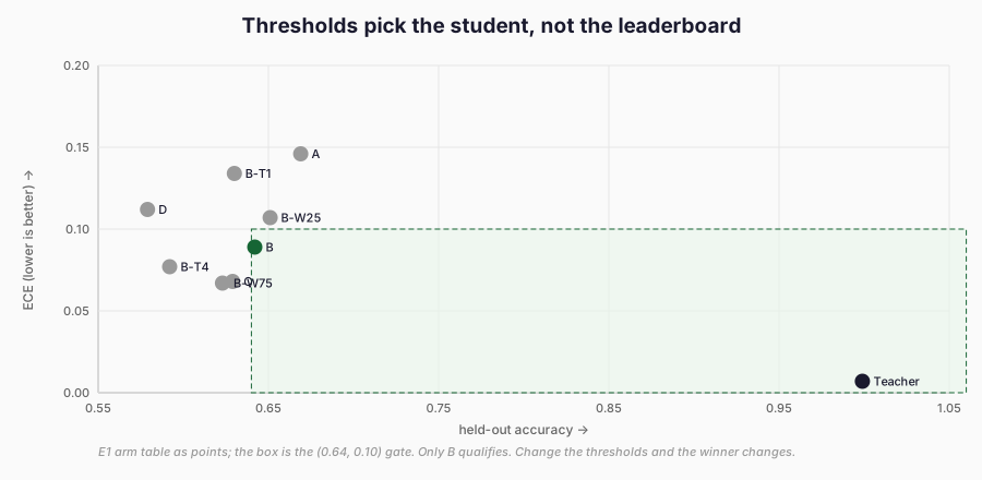
Figure 1. The E1 arms as points: only B among students sits inside the (≥0.64, ≤0.10) box (the teacher is the reference, not a candidate). Change the thresholds and the winner changes — the procedure, not the name, is the contribution.
The winner on accuracy alone (A) fails the calibration gate; the constrained optimum among students is B, the mixed-distillation arm — chosen not for being “distilled” but for satisfying both constraints, with the teacher as the reference point no student touches. Note the asymmetry the procedure exposes: A leads B by 0.027 on accuracy and trails by 0.057 on ECE — the accuracy gap is narrower than the calibration gap, which is exactly why a single-metric ranking and a two-constraint rule disagree, and why the rule is the more honest description of what deployment wants.
This is the book’s recurring lesson in selection form: Chapter 05’s calibration trade-off (mixed KD lower ECE, lower accuracy) becomes, under explicit thresholds, a decision procedure. Change the ECE cap to 0.15 and A becomes eligible; since costs tie within E1, it wins only on an accuracy tie-break, which the rule must then state. The chapter’s contribution is the procedure, and the table that makes the threshold-dependence visible, not the name of the winner. Add a latency cap of 0.05 ms and the field narrows differently: both E1 candidates survive it (0.018 and 0.011 ms), the E2 teacher does not (0.055 ms), and among E1 students the accuracy ordering is unchanged — the cap binds the family choice, not the arm choice. Thresholds compose, and each added constraint can only shrink the qualifying set — which is why the chapter records qualifying sets rather than winners: the reader replays the rule with their own numbers, and the book’s numbers are one instantiation, not a leaderboard.
Worked example — three small students, no monotonicity
Take three tiny models and one host. The 228-parameter E1 student answers in 0.011 ms (batch 1); the 370-parameter router in 0.012 ms; the 1,200-parameter direct-answer policy in 0.012 ms; the 1,140-parameter signal MLP in 0.017 ms. Ordered by latency: e1-student < e4-answer ≈ router < signal-mlp. Ordered by parameters: e1-student < router < signal-mlp < e4-answer. The orderings disagree — 1,200 parameters answer as fast as 370, and 1,140 slower than both — because latency at this scale is operator mix and framework overhead, not parameter count.
None of these numbers compares capability (four different tasks); all of them compare cost, and cost alone already refutes “fewer parameters means faster”. A Pareto frontier over these cost axes alone would keep only the e1-student, which is no worse than the other three on any measured cost. That answer is useless, because the four models do different jobs. It shows the method’s limit: without a correctness axis, Pareto ranks price, not fitness for the task.
The cross-architecture cost catalog
Fourteen architectures, one protocol, one host. The numbers that carry the chapter’s argument:
- The e4-tool policy holds 10,400 parameters — 2.6× the e3-student’s 3,984 — and answers in 0.012 ms against 0.140 ms: an order of magnitude faster with two-and-a-half times the weights. An MLP over 64 inputs is not a smaller transformer; it is a different computation, and the parameter ratio points the wrong way.
- The E1 teacher is 76× the E1 student’s parameters (17,412 vs 228) and 1.6× its batch-1 latency (0.018 vs 0.011 ms): at batch 1 both are overhead-bound, and the 76× buys almost no time and costs 69,648 vs 912 bytes on disk.
- Batch 32 changes every ranking it touches: e2-student latency grows 0.043 → 0.225 ms (5.3× for 32× work — genuine throughput, 142k examples/s), while e1-student grows 0.011 → 0.012 ms (overhead-bound; throughput 2.6M/s is arithmetic, not achievement). The difference is arithmetic intensity: the convolutional student does enough multiply-adds per byte loaded that batching amortises the framework overhead, while the tiny MLPs finish each batch before the overhead notices and 32× work costs 1.1× time. Neither regime is “better” in the abstract — a serving system that batches pays for throughput, one that cannot batch pays for single-example latency, and the two optima differ. A serving decision made at batch 1 reverses at batch 32 for the convolutional pair and barely moves for the MLPs — which is why the protocol fixes batch sizes instead of reporting “latency”.
- The transformer students scale with sequence and width together: struct-student (4,464 params, 32-length rows) at 0.153/1.207 ms vs e3-student (3,984 params, 24-length rows) at 0.140/0.767 ms. Same family, same operators, longer rows and a larger head: cost follows the workload signature, and the signature is part of every record so the comparison can be audited.
- Peak process memory spans 379.9–389.7 MB across all fourteen — a 10 MB range on a ~380 MB runtime. The methodology note matters more than the numbers: process high-water mark cannot resolve model memory at this scale (the largest checkpoint here is 111 KB), so the chapter reports it as a bound (“fits comfortably”) and refuses to rank by it. Model memory would need allocator-level accounting the study does not perform — recorded as NOT MEASURED, not estimated from parameter count.
Per-family Pareto: distillation does not change the price tag
Each family’s students share one deployment architecture, so costs tie within a family by construction and the Pareto computation verifies it mechanically:
- E1: frontier {A, teacher}. Every distillation arm is dominated on accuracy at identical cost; the teacher sits on the frontier by being better at everything except cost (0.999 mean held-out accuracy over three seeds against the students’ 0.58–0.67). Within-family, distillation is pure accuracy movement at fixed price.
- E2 (with the extension arms): frontier {F-relational-distance, teacher}. The relational arm’s mean gain of nearly six points over the baseline (0.934 vs 0.877) is the largest student improvement in any family compared here — at exactly the same deployment cost (372 parameters, same forward pass; the relations were a training signal, with no projector kept for inference, unlike the feature arms whose projector is training-only in any case). Including the extension arms is legitimate because they share the task, splits, seeds, and student architecture of the base E2 study — the manifest records A–D means reproduced exactly — so the frontier spans two runs of one protocol rather than two protocols.
- E3-transformer: frontier {B-token-kl, teacher}. The mixed KL arm edges the baseline (0.528 vs 0.525) at identical cost.
- E3-structured: frontier {C-filtered, teacher}. Verification filtering edges the oracle baseline (0.402 vs 0.391) at identical cost.
- E4-agent: the computation returns {A-answer-only} — cheapest at zero success everywhere. This is the formalism working as designed and the decision it returns being absurd, which is why the chapter states it plainly: a Pareto frontier over a capability axis with no separation is not a recommendation. The mission’s promotion-gate pattern (Chapter 36/42) exists for exactly this case: first a minimum-capability threshold, then Pareto among the survivors. No E4 arm clears any non-zero bar, so no E4 student is selectable — the method refuses where a naive ranking would crown the cheapest zero.
The pattern across families is the chapter’s central empirical claim, and it is strong precisely because it is boring: in no family does the distillation method change the deployment profile. Fewer parameters were never on offer — the same student, trained differently. The one cost difference inside a family, E4’s smaller answer-only baseline, comes from a different policy design, not from a distillation loss. Latency, memory, and storage are architecture properties, fixed before the teacher’s first forward pass. What distillation buys, at most, is movement along the correctness axis inside a cost envelope someone else chose. Anyone selling distillation as compression is selling the envelope, not the training.
Rejected candidates: tokenizers and licences
Two rejections the chapter records rather than performs. First, a tokenizer mismatch: the E3 instruction rows (vocab 9) cannot be fed to the structured JSON student (vocab 20) or vice versa — the logit tensors do not align, and the runner refuses instead of projecting silently (the tested pattern from Chapter 17). A student that cannot read the deployment tokenizer at the same ids is not a smaller student; it is an incompatible one, and no Pareto table should contain it. Context length is the quieter tokenizer cost: the struct-student’s 32-token rows cost 0.153/1.207 ms against the e3-student’s 24-token rows at 0.140/0.767 ms — same family, same operators, longer rows. The workload signature in every record exists so that a deployment with 128-token prompts does not inherit a 24-token measurement without noticing.
Second, a licence screen: the repository’s own models are self-created under its Apache-2.0 licence, but a real selection would screen candidates such as Qwen3-0.6B (declared Apache-2.0, L-006 — permissive, attribution required) against gated alternatives (the gated Gemma card, L-013, which carries the Gemma terms and their derivative conditions; the gated Llama card, L-014, which carries the Llama terms and their naming and scale conditions). A gated candidate that cannot be fetched cannot be benchmarked, and a licence that restricts redistribution can dominate the technical Pareto without appearing in it. Both rejections are prose fixtures with the mechanism stated (refuse, record, exclude) — the chapter’s contribution is the gate in the selection procedure, not the outcome of any particular screen.
Cost, stability, and rights
Training cost is cited from frozen records as reference, not re-measured: E1 students ~6–8 s, E2 ~3 s, E3-transformer ~17 s, E3-structured ~15 s, E4 policies ~1–3 s per arm per seed (all host-sensitive, all single-host CPU). The new measurements cost seconds total (0.4 s wall for all fourteen candidates) because no training occurs — inference benchmarking is cheap, which is why there is no excuse for selecting on parameter count instead of measuring.
Stability across repetitions is reported as p95 alongside the median (tails exceed medians by up to ~2× across candidates; the largest ratio is the convolutional E2 student’s at batch 1, with the transformer rows next — batch-1 scheduling jitter on sub-millisecond workloads, not model pathology), and the single-day, single-host scope is stated on every number: these transfer as methodology, not as universal constants.
The study uses RM-123, VERIFIED_PERMITTED for
benchmark_inference_architectures. All architectures are
self-created; all weights fresh random inits; no training data,
external models, checkpoints, or personal data involved. Correctness
figures are read from frozen verified manifests, never recomputed —
the record that makes the Pareto analyses reproducible without
re-running a single student. Student licences for deployment follow
the repository’s Apache-2.0 terms for its own code, with the
per-experiment rights records (RM-101 through RM-122) governing
teachers, data, and outputs; export control, data residency, and
product-specific use restrictions are flagged as deployment-time
questions for specialist review, not answered here.
Concretely, a deployment that ships weights across a border, serves queries containing personal data, or embeds the student in a regulated device would each need its own determination — jurisdiction, lawful basis, and product classification respectively — and none of them is settled by a latency table, however carefully measured. The licence and deployment record the contract requires is therefore a pointer to open questions with owners, not a certificate: model licence recorded, teacher/data rights referenced by record id, export and residency flagged undecided. RM-104 and all prior records are untouched.
Limitations
One host, one CPU thread, fp32 only — no GPU, no quantised runtimes, no kernels. Fourteen architectures but one workload each; sequence length and batch size vary only where the protocol varies them — a candidate whose cost explodes at long contexts looks identical here to one that does not, and the workload signatures exist precisely so that a deployment outside them re-measures instead of inheriting. FLOPs not computed (deliberately; latency measured instead).
Model memory not isolated from process memory (methodology bound, not a ranking). Frozen correctness spans unrelated tasks and is never ranked across families; teacher points for E3 families use validation accuracy against student test accuracy (disclosed mismatch, same generator). All E2 extension arms were included (shared task, splits, seeds, and student), but no E4 Pareto is recommended and no cross-task ranking is performed, by design rather than by omission. No external replication and no independent review.
Preparing for efficient training
Selection assumed the student already exists. Chapter 32 asks what happens when training itself is the scarce resource: can the same behaviour be distilled while updating far fewer parameters? The benchmarking interface built here — costs, workloads, methodology records, Pareto membership — is the instrument that chapter will reuse, because a LoRA adapter’s claim (“same capability, fewer trainable parameters”) is exactly the kind of claim that needs a cost ledger rather than a parameter count. The frontier computed above is the baseline it must beat: same deployment cost or it does not count as efficiency, no matter how small the trainable fraction.
References
Cho, J. H. and Hariharan, B. (2019). On the Efficacy of Knowledge Distillation. Proceedings of the IEEE/CVF International Conference on Computer Vision (ICCV). arXiv:1910.01348. https://arxiv.org/abs/1910.01348
Mirzadeh, S. I., Farajtabar, M., Li, A., Levine, N., Matsukawa, A. and Ghasemzadeh, H. (2020). Improved Knowledge Distillation via Teacher Assistant. Proceedings of the AAAI Conference on Artificial Intelligence. arXiv:1902.03393. https://arxiv.org/abs/1902.03393
Legal sources
Qwen3-0.6B model card. Last modified 26 July 2025. https://huggingface.co/Qwen/Qwen3-0.6B (retrieved 12 November 2026). Cited as L-006 for the Apache-2.0 licence context in candidate screening; not legal advice.
Gemma 3 1B IT model card. Last modified 4 April 2025. https://huggingface.co/google/gemma-3-1b-it (retrieved 12 November 2026). Cited as L-013 for the gated-access and Gemma-licence context in candidate screening; not legal advice.
Llama 3.2 1B Instruct model card. Last modified 24 October 2024. https://huggingface.co/meta-llama/Llama-3.2-1B-Instruct (retrieved 12 November 2026). Cited as L-014 for the naming, notice, and acceptable-use context in candidate screening; not legal advice.