Attention and Relational Distillation
Structure can transfer without copying values: spatial attention maps, pairwise distances, triplet angles, and similarity matrices. This chapter derives those objectives, shows their invariances and batch dependence, and reports a controlled E2 extension.
In this chapter’s experiment, a student trained to keep its teacher’s pairwise distances finished with mean accuracy 5.63 percentage points above a student trained on labels alone, the largest difference among the seven arms. Most of that difference came from one of the three seeds. The distance error the student was trained to reduce did fall, but that is what optimising it should do; it is a consistency check, not evidence that the preserved structure caused the gain. Relational supervision is promising here and fragile here, and this chapter keeps both observations in view.
Chapter 08 matched feature values through a projection. A student that reproduces the teacher’s coordinates more closely is rewarded, whether or not those coordinates matter for the task. This chapter asks a different question:
Can the student learn the relationships the teacher represents, rather than only the teacher’s per-example outputs?
The answer is a qualified yes, with two conditions. First, the relation has to be defined precisely: which layer, which aggregation, which normalisation, which pairs or triplets, which reduction. Second, the evaluation has to separate the relation from the task. A smaller relational loss is evidence that structure was preserved. It is not evidence that the student is more correct.
Relational distillation (KD-013) is supervision from relations between examples or representations rather than from individual values alone. Attention transfer and relational distillation are related but not identical: attention transfer compares spatial maps within each example, while relational losses compare examples with each other inside a batch.
From copying features to copying structure
Pointwise feature matching says: for this input, make this vector equal to that vector. Relational matching says: for these inputs, keep the same distances, angles, or similarities that the teacher keeps. The difference matters when the spaces differ. A teacher with 32 channels and a student with 8 channels cannot share coordinates, but both can define a 64-by-64 distance matrix on the same minibatch. The matrix has the same shape even though the underlying spaces do not.
Structure is also more invariant than coordinates. Translating every feature by the same vector leaves pairwise distances unchanged. Rotating every feature leaves distances and angles unchanged. Multiplying every feature by a positive constant leaves normalised distances and angles unchanged, and leaves cosine similarity unchanged. A student that preserves relations can therefore differ from its teacher in ways that pointwise MSE would penalise. Whether that freedom helps depends on the task and on how the relations are measured.
The cost of that freedom is batch dependence. A distance matrix, an angle set, and a similarity matrix are all functions of the comparison set. Change the minibatch and the target changes, even for identical examples. Relational training therefore couples the objective to data loading in a way that pointwise losses do not.
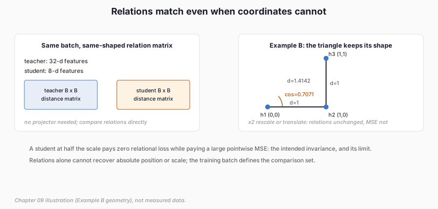
Figure 1. Why relations transfer across mismatched spaces. A 32-dimensional teacher and an 8-dimensional student define same-shaped batch relation matrices; the triangle shows the Example B geometry whose normalised distances and angles survive rescaling and translation. Chapter illustration, not measured data.
Attention maps from CNN activations
For a convolutional feature map
A concrete map makes the operation visible. Take a single example with two channels on a \(2\times2\) grid:
Attention-transfer mathematics
Let \(Q_S^j\) and \(Q_T^j\) be the flattened student and teacher attention maps for layer pair \(j\). Let \(\hat q_S^j\) and \(\hat q_T^j\) be the L2-normalised flattened maps with \(M_j=H_jW_j\) spatial positions. The transfer loss used here is the mean over maps and, within each map, over spatial positions (and over batch elements in the implementation, where the code averages all squared differences):
Normalisation is the point: without it, a student with larger activations would pay a larger loss for the same spatial pattern. With it, only the shape of the map matters. The teacher map is detached; gradients flow through the student only. The implementation rejects spatial mismatches instead of silently interpolating, because resampling changes the meaning of the comparison.
The gradient follows from the normalised difference by the chain rule through the aggregation and normalisation. The tests check it against autograd and against a central finite difference. For the E2 block2 pair, teacher \([B,32,6,6]\) and student \([B,8,6,6]\) both yield \([B,6,6]\) maps, so no projector is needed. That is the practical advantage over Chapter 08: attention transfer compares spatial maps, not channels.
Example A. Using the two-channel map above as the teacher and
Gradient-based attention and why it is omitted
Zagoruyko and Komodakis also define a gradient-based map: the gradient of the loss with respect to the input, treated as an input-sensitivity map, with an optional horizontal-flip symmetry term. Training a student to match it requires a second backpropagation through a mixed partial derivative, roughly doubling the backward cost, and its behaviour under batch normalisation is subtle because the normalisation statistics participate in both passes. The E2 extension does not implement gradient-based transfer. Activation-based transfer is cheaper, better matched to the available feature interface, and sufficient to demonstrate the spatial-structure idea. Omitting the gradient variant is a scope decision, not evidence against it.
Why attention is not an explanation
An attention map highlights where activations are large. It does not say that those positions caused the prediction, that the model reasoned about them, or that a human would find them meaningful. Two networks can produce similar maps for different reasons; two accurate networks can attend to different regions. Normalisation discards magnitude, aggregation discards channel identity, and the map discards everything outside the chosen layer.
The chapter therefore treats visual comparison as inspection, not evidence. A map may help debug a collapsed student or a misaligned layer. It cannot show that the student reasons like the teacher, and a prettier map is not a better classifier. Chapter 35 returns to misleading interpretability claims as a failure mode.
Pairwise relational distances
For a minibatch of representations \(h_1,\ldots,h_B\in\mathbb R^d\), define
The distance loss (RKD-D) is a Huber penalty between normalised teacher and student distances:
Because only relations are compared, teacher and student may have different feature dimensions. In E2 the pooled teacher vector has 32 dimensions and the student has 8; no projector is used for the relational arms.
Triplet relational angles
For distinct examples \(i,j,k\) with anchor \(j\), define unit directions
Enumerating every ordered triplet costs \(O(B^3)\). The implementation takes an
explicit triplet list instead. Training uses 128 deterministically sampled
triplets per batch with seed seed + epoch * 1000, matching the executed
code (e2_extension_09.py:197; the batch count 128 is recorded in the
manifest). The sampling budget is therefore fixed and reproducible. Sampling more triplets
covers more structure at higher cost; sampling fewer leaves structure unseen.
Neither choice is neutral, and the budget belongs in the protocol.
Example B. Take three two-dimensional points
Similarity-preserving objectives
Tung and Mori (2019) compare pairwise similarities instead of distances. For a batch matrix \(H\in\mathbb R^{B\times d}\),
The three relational objectives differ in what they keep. RKD-D keeps normalised pairwise distances; it is insensitive to translation, rotation, and global scale but sensitive to the batch mean used as normaliser. RKD-A keeps triplet angles; it adds rotation invariance around the anchor and is insensitive to the same global transforms, at the cost of cubic triplet growth without sampling. Similarity preservation keeps row-normalised Gram structure; it is sensitive to translation and rotation in general because the raw dot product is, and removes scale only through the row norm. None of them requires a feature projector, which is their practical advantage over Chapter 08. None of them is a substitute for the others without an ablation.
Invariances and what they cost
| Objective | Pointwise | Translation | Rotation | Positive scale | Batch order | Feature dim |
|---|---|---|---|---|---|---|
| Feature MSE | exact match | sensitive | sensitive | sensitive | independent | must match |
| Feature cosine | direction | sensitive | sensitive* | invariant | independent | must match |
| Attention transfer | map shape | sensitive | sensitive | invariant† | independent | channels free |
| RKD distance | relations | invariant | invariant | invariant | dependent | dims free |
| RKD angle | relations | invariant | invariant | invariant | dependent | dims free |
| Similarity (SP) | relations | sensitive | sensitive‡ | invariant | dependent | dims free |
* Cosine is invariant to a common positive scale but not to rotation in general; the table records uniform-configuration transforms. † After L2 normalisation; raw maps are scale sensitive. ‡ Unnormalised dot products are scale and rotation sensitive; row normalisation removes scale only.
Normalisation is what creates invariance, and every normalisation discards something. Distance normalisation discards global scale. Angle computation discards scale and translation. Attention normalisation discards map magnitude. Row-normalised similarity discards absolute activation scale. None of these choices is free, and none makes two different architectures semantically identical.
Batch composition and cost
Relational losses are functions of the comparison set. The same example receives a different target depending on its neighbours. A balanced batch, an unbalanced batch, a small batch, and a large batch define different distance means, different triplet populations, and different normalisers. This is both the mechanism and a source of instability: relations expose batch structure, but they also inherit batch noise.
Complexity matters. Pairwise distances are quadratic in batch size. Exhaustive triplets are cubic. Deterministic sampling bounds the cost but covers only part of the structure. Memory grows with the batch and with the stored teacher features. The E2 extension fixes batch size 64 for training, samples 128 triplets per batch, and reports the sampling budget explicitly.
A rough accounting makes the trade-off concrete. For batch 64 and feature dimension \(d\), the distance matrix holds \(64^2=4{,}096\) scalars regardless of \(d\). The angle computation touches 128 triplets per batch, each a dot product in \(d\) dimensions, rather than all \(\sim\)250,000 ordered triplets. Attention transfer adds one forward aggregation and one normalised MSE per layer pair, with no projector and no pairwise matrix. The projector, where present, is the dominant extra cost: 288 parameters for the E2 1x1 convolution, against a 372-parameter student. Relational arms avoid the projector entirely but pay the batch-quadratic or sampled-cubic comparison instead. Which cost is smaller depends on the batch size, the feature dimension, and the number of sampled triplets; the manifest records all three so the comparison is explicit.
Example C. On frozen validation features with fixed models, the same teacher–student pair gives different relational losses under different compositions. In the E2 extension diagnostic:
| Composition | Batch | RKD-D | RKD-A |
|---|---|---|---|
| Balanced | 64 | 0.0698 ± 0.0071 | 0.0752 ± 0.0109 |
| Unbalanced | 64 | 0.0728 ± 0.0102 | 0.0780 ± 0.0123 |
| Small | 16 | 0.0577 ± 0.0165 | 0.0805 ± 0.0188 |
| Large | 128 | 0.0662 ± 0.0079 | 0.0817 ± 0.0147 |
Each entry is five repeats on validation data only. The models are fixed, so the differences come from the comparison set, not from training. Identical examples receive different relational signals in different minibatches. A training batch-size sweep would confound this with optimisation effects, so it is omitted; the frozen analysis isolates composition from training.
Two leakage rules apply to any such diagnostic. First, never mix splits when constructing compositions: the validation features used here come from one split, and test features are never used to choose a composition. Second, do not let relational statistics leak across the train/validation boundary during selection. The diagnostic runs after training on frozen models and fixed validation features; it does not update any weight and does not inform checkpoint selection.
The controlled E2 extension
The extension reruns A–D under the identical E2 protocol, data, seeds, optimiser, budget, and selection rule, and adds E–G. Historical E2 values are preserved separately; the seven-arm table below is one controlled run, not a merge of old and new numbers.
| Arm | Objective |
|---|---|
| A-hard | Ground-truth cross-entropy |
| B-output-kl | CE + 0.5 · \(T^2\) KL, \(T=2\) |
| C-feature-mse | CE + 0.5 · projected feature MSE |
| D-feature-cosine | CE + 0.5 · projected feature cosine |
| E-attention | CE + 0.5 · attention transfer (block2, \(p=2\)) |
| F-relational-distance | CE + 0.5 · RKD-D on pooled block2 |
| G-relational-angle | CE + 0.5 · RKD-A on pooled block2 |
Attention uses block2 maps directly (\(32\times6\times6\) vs \(8\times6\times6\));
no projector is needed because channels are aggregated away. Relational arms
use global-average-pooled block2 vectors (teacher 32-d, student 8-d) with no
projector. Coefficients are fixed at 0.5 for comparability with E2, not tuned
to the test set. Triplet sampling is 128 per batch with seed seed + epoch * 1000, matching the executed code.
The teacher was retrained under the same configuration and seeds. It reached 99.4–99.5% test accuracy, matching E2. All arms ran 40 epochs with patience 8 and ground-truth validation selection.
| Arm | Accuracy (%) | CE | ECE | Agreement (%) | Probe (%) |
|---|---|---|---|---|---|
| A-hard | 87.73 ± 8.96 | 0.3604 ± 0.2223 | 0.1016 ± 0.0358 | 87.57 ± 9.06 | 86.07 ± 9.27 |
| B-output-kl | 88.37 ± 7.28 | 0.3132 ± 0.1841 | 0.0650 ± 0.0307 | 88.33 ± 7.48 | 85.57 ± 8.32 |
| C-feature-mse | 89.07 ± 8.32 | 0.3864 ± 0.1846 | 0.1436 ± 0.0211 | 89.07 ± 8.52 | 86.70 ± 9.53 |
| D-feature-cosine | 88.73 ± 7.90 | 0.3682 ± 0.2200 | 0.1240 ± 0.0469 | 88.73 ± 8.05 | 86.53 ± 9.39 |
| E-attention | 89.43 ± 6.52 | 0.3143 ± 0.1844 | 0.0939 ± 0.0386 | 89.47 ± 6.82 | 86.43 ± 8.11 |
| F-relational-distance | 93.37 ± 7.59 | 0.2434 ± 0.2249 | 0.0964 ± 0.0630 | 93.30 ± 7.71 | 91.47 ± 8.39 |
| G-relational-angle | 92.87 ± 8.04 | 0.2747 ± 0.2458 | 0.1140 ± 0.0665 | 92.83 ± 7.91 | 91.60 ± 9.13 |
Per-seed accuracy shows the spread behind the means:
| Seed | A | B | C | D | E | F | G |
|---|---|---|---|---|---|---|---|
| 0 | 0.790 | 0.820 | 0.796 | 0.809 | 0.832 | 0.846 | 0.836 |
| 1 | 0.873 | 0.868 | 0.924 | 0.886 | 0.889 | 0.979 | 0.980 |
| 2 | 0.969 | 0.963 | 0.952 | 0.967 | 0.962 | 0.976 | 0.970 |
A–D reproduce the historical E2 means exactly, confirming that the new run is comparable. The relational arms show the largest mean differences (F +5.63 pp, G +5.13 pp over A), but seed 1 carries most of the effect and the spread is 7–8 pp. Attention is +1.70 pp with the lowest CE among the structural arms.
Relational diagnostics on the test set (means over seeds):
| Arm | Attention loss | RKD-D error | RKD-A error |
|---|---|---|---|
| A-hard | 0.0052 | 0.0754 | 0.1127 |
| E-attention | 0.0031 | 0.0719 | 0.1067 |
| F-relational-distance | 0.0042 | 0.0446 | 0.0706 |
| G-relational-angle | 0.0037 | 0.0403 | 0.0683 |
F and G reduce the relational errors they directly optimise, as expected. That is a consistency check, not proof that the relation caused the accuracy difference.
What improved and what did not
F and G improved mean accuracy, mean CE, and mean probe accuracy relative to A on this task and budget. E improved mean accuracy and CE modestly. But the evidence is weaker than the headline differences suggest:
- Three seeds cannot support a significance claim; seed 1 dominates F and G.
- C and D have higher CE and ECE than A despite higher mean accuracy.
- F and G have lower CE than A but higher ECE than B.
- The probe improves for F and G (+5.4 and +5.5 pp over A) but remains within a large spread and does not isolate which structure mattered.
- Attention maps were not evaluated as explanations, and no claim is made that E looked at the right regions.
- No coefficient, layer, or batch-size sweep was performed; different settings could change the ordering.
The honest summary is a qualified positive for relational supervision on this task, not a general advantage. Feature arms C and D remain near baseline; the structural arms E–G move further, with relational arms moving most. The batch diagnostic explains part of why: relational targets shift with composition, so the training signal is richer but noisier than a fixed per-example target.
Rights and operational constraints
Attention maps, pooled features, distances, angles, and similarity matrices are derived from model weights and inputs. They can expose training or user information and may be subject to confidentiality, personal-data, or contractual constraints. A hosted API generally does not expose intermediate features; the fact that a local open-weight teacher does is an interface property, not permission.
The extension used only self-created images and models under RM-103, which
authorises train_and_evaluate_e2. The same action string covers this
extension because the data source, model family, local execution, and
non-distribution conditions are unchanged. The runner invoked the existing gate
and would have refused to train on failure. RM-101 and RM-102 are unchanged.
Chapters 36–39 carry the full legal framework; this chapter records the
interface and the intended action and blocks when the answer is unknown.
Operationally, the projector is training-only for C and D (288 parameters, excluded from the 372-parameter deployment student). Attention and relational arms use no projector. Teacher features are detached in every arm; student and projector gradients flow. Training time was 1.9–5.3 s per arm-seed for A–G in the extension run; peak memory is a cumulative process diagnostic, not model-only memory.
Preparing for sequence-level distillation
Outputs, restricted outputs, features, maps, and relations all concern one input at a time or batches of independent inputs. Chapter 10 changes the unit of supervision to entire sequences. A generated sequence is a structured object with order, length, and autoregressive dependence; matching it raises tokeniser, alignment, exposure-bias, and rights questions that do not arise here. The discipline carries over: define the signal, record the access, derive the objective, measure correctness independently, and keep similarity diagnostics separate from task success.
References
Park, W., Kim, D., Lu, Y. and Cho, M. (2019). Relational Knowledge Distillation. Proceedings of the IEEE/CVF Conference on Computer Vision and Pattern Recognition (CVPR), pp. 3967–3976. https://arxiv.org/abs/1904.05068
Tung, F. and Mori, G. (2019). Similarity-Preserving Knowledge Distillation. Proceedings of the IEEE/CVF International Conference on Computer Vision (ICCV), pp. 1365–1374. https://arxiv.org/abs/1907.09682
Zagoruyko, S. and Komodakis, N. (2017). Paying More Attention to Attention: Improving the Performance of Convolutional Neural Networks via Attention Transfer. International Conference on Learning Representations (ICLR). https://arxiv.org/abs/1612.03928