The Data Behind the Knowledge
Distillation is only as sound as its data: origin, identity, splits, contamination, coverage, and permission. This chapter defines dataset provenance, builds a manifest, and retrospectively audits the E1 and E3 precursor datasets without rerunning them.
One field in the E3 experiment’s manifest records 1,200 teacher-generated targets. The experiment generated 3,600: 1,200 for each of three seeds, with the field keeping only the count from the final seed’s loop. Nothing in a training curve would reveal the difference. Only an audit of the records does, and an audit can only find what the records kept. This chapter is about keeping the records that make such an audit possible.
Part II asked how a student should learn from a teacher. Part III asks a prior question: what exactly was the student shown, where did it come from, and were we permitted to use it? A mathematically correct training procedure can still produce misleading results if its data is contaminated, poorly specified, or used without permission.
The central question is:
What must be true of the data for a distillation experiment to be meaningful, reproducible, and lawful?
The answer this chapter defends is that the knowledge available for distillation depends on the examples used to teach the student, and those examples must have a known origin, controlled transformations, valid training/evaluation separation, appropriate coverage, and permission for their intended use. None of this is visible in a loss curve.
Data carries the knowledge
Every distillation result in this book was produced by showing a student a particular collection of examples. The E1 student saw 1,200 synthetic spiral points per seed; the E3 precursor student saw 1,200 synthetic symbol strings per seed plus teacher-generated targets. Change those collections — duplicate them, leak the test inputs into training, quietly substitute a different generator version — and the measured numbers change while the code stays identical. The data is not the backdrop of the experiment. It is the supervision itself, in its most concrete form.
That is why data handling deserves the same engineering discipline as loss design. A dataset needs an identity (which dataset, which version), a history (who made it, what changed), a boundary (what belongs to training versus evaluation), and a licence (what may be done with it). Missing any one of these turns a measured result into an anecdote: accurate, perhaps, about some computation that happened once, but not reproducible and not auditable.
Why data provenance matters
Data provenance (KD-041) is the recorded origin, transformations, rights, and chain of custody of data used in a learning system. It answers four distinct questions that are often collapsed into one vague appeal to “the dataset”:
- Source identity. Which artefact, exactly — name, version, creator, retrieval date? A URL is a lookup hint, not an identity: the content behind it can change.
- Ownership or control. Who decides what the data may be used for? Availability is not authority; a downloadable file is not a permitted file.
- Legal permission. What action is allowed — training, evaluation, redistribution, competing-model development? Permission is action-specific: approval to evaluate is not approval to train on.
- Lineage. What transformations produced this exact set from its sources — generation code and its hash, configuration and its hash, seeds, split assignments, filtering decisions, teacher decoding that produced derived targets?
A dataset may be reproducible without being lawfully usable (exact bytes, no permission). It may be legally usable without being representative (full permission, narrow coverage). It may have perfect checksums and still contain evaluation leakage (integrity of bits, not of boundaries). Each property needs its own record, because each can fail independently.
Dataset identity and versions
Six different things travel under the name “dataset”, and an audit must keep them apart:
- A named dataset (“the E1 spiral set”).
- A particular version of it (“protocol 1.0, noise 0.08”).
- The implementation that generates it (source file plus its hash).
- The configuration (sizes, seeds, noise, split offsets, plus its hash).
- The exact examples produced (bytes, plus their hash).
- The train/validation/test partition assignments (which row went where).
A source-code hash is not a content hash: the same program with a different seed produces a different dataset, and the same seed under a changed random-number implementation can too. A generation seed is therefore necessary but not sufficient; it must be paired with the code hash. Conversely, a content hash tells you what you have but not how it was made; it must be paired with the generator identity.
The convention used in this book is SHA-256 throughout: canonical JSON (sorted keys, compact separators) for configurations, length-prefixed canonical row encodings for content (so concatenation can never blur row boundaries), and an explicit statement of whether a hash is order-sensitive (dataset identity) or order-insensitive (duplicate detection support).
Deterministic regeneration is the practical test. If the recorded code, configuration, and seed reproduce the recorded fingerprint byte for byte, the dataset is reproducible from its documentation. The E1 audit below passes this test for all three seeds; so does the E3 audit. What neither audit can do retrospectively is prove that the historical run executed that code path — the fingerprint match confirms the records describe the data, not that the data was used as described. That distinction runs through the rest of the chapter, and the closing section, “Lessons and limits of the audits”, states it plainly.
The dataset manifest
A dataset manifest is the single record that binds identity, history,
boundaries, and permission. The implementation in this chapter
(DataManifest in examples/common/provenance.py) is deliberately flat:
plain dataclasses serialised to canonical JSON, validated by a small
explicit checker, with no database, catalogue service, or workflow engine
behind it. It records:
- Dataset identifier, version, and plain-language description.
- Creator or source, source type, and creation or retrieval date.
- Source version and the rights record plus the authorised action.
- Generator identity, generator hash, configuration hash, and seed.
- Sample count, input and target schemas, transformation history.
- Per-split identities: name, count, fingerprint, generation rule, seed offset.
- Known limitations and a validation status.
Validation is mechanical: every required field present, split counts summing to the sample count, unique split names, non-negative counts. Anything interpretive — whether the coverage is adequate, whether the rights record covers a new action — is left to the reader and the rights gate, not to the schema. A manifest that validates is complete, not correct; completeness is checkable, correctness is a judgment.
    flowchart LR
  G[generator + code hash] --> R[raw examples + content hash]
  R --> S[splits by rule + fingerprints]
  S --> T[teacher targets + decoding config]
  T --> M[manifest binds all + rights record]
  M --> U[student use or block]
Figure 1. The chain of custody as one linked record: each stage names its inputs’ hashes, and the manifest binds them before any training.
Training, validation, and test distributions
Let the intended task distribution be \(P_{\mathrm{task}}(X,Y)\): the inputs and labels the deployed student will actually face. The empirical training distribution is
\[ \hat P_{\mathrm{train}}(X,Y)=\frac{1}{n}\sum_{i=1}^{n}\delta_{(x_i,y_i)}, \]
the uniform mixture over the \(n\) training examples. Evaluation happens under \(P_{\mathrm{eval}}(X,Y)\), the distribution the test set samples. Three distributions, three different roles: the task is what we care about, the training set is what we optimise, and the evaluation set is what we measure. A result is only as meaningful as the alignment between them.
Sampling variation is the first wedge. A finite training set approximates the task distribution, and its quirks — which regions are dense, which are absent — become part of what the student learns. The E1 training spirals are smooth and balanced; a student that masters them has mastered smooth balanced spirals, nothing more.
Covariate shift is the standard setting \(P_{\mathrm{train}}(X)\ne P_{\mathrm{eval}}(X)\) with the conditional relationship held stable, \(P_{\mathrm{eval}}(Y\mid X)\), wherever both are supported. The inputs move; the labelling rule does not. A student evaluated on inputs unlike its training inputs is being asked to extrapolate, and its test score measures extrapolation, not competence.
Label shift reverses the pattern: \(P_{\mathrm{train}}(Y)\ne P_{\mathrm{eval}}(Y)\) while \(P_{\mathrm{eval}}(X\mid Y)\) stays stable. Class proportions change; the appearance of each class does not. A balanced training set evaluated on a skewed deployment is a label-shifted evaluation, and accuracy will move for purely statistical reasons. A toy calculation makes the point: a classifier correct on 90% of class A and 60% of class B scores 75% on a balanced test set but only 63% when class B is 90% of deployment — same model, same per-class behaviour, twelve points of “regression” from composition alone. E1’s uniform class balance is therefore a choice with consequences: it measures per-class competence evenly, at the cost of saying nothing about skewed deployments.
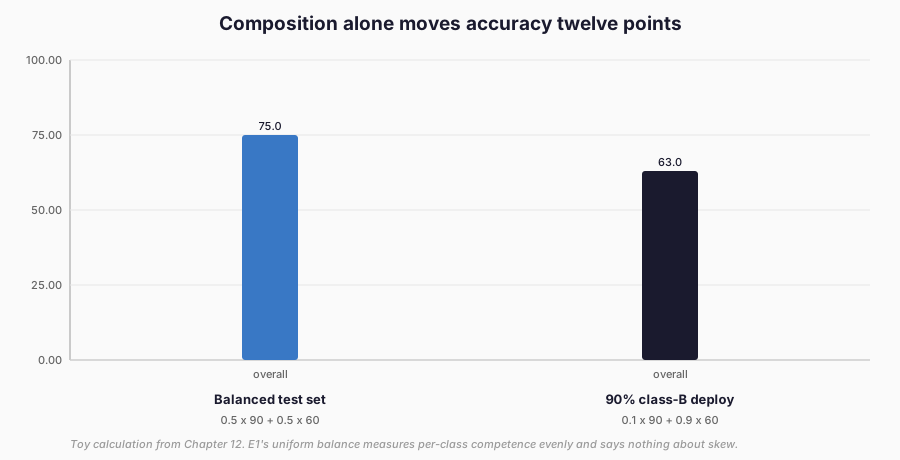
Figure 2. The toy calculation drawn as bars: identical per-class behaviour (90% on A, 60% on B) scores 75% balanced but 63% under 90% class-B deployment. Toy arithmetic, not a measurement.
Concept change is the harder case: the relationship itself differs, and neither conditional can be assumed stable. Do not label every observed difference “covariate shift”; the name carries an assumption about what stayed fixed, and the assumption needs evidence. The honest statement in most applied settings is the weakest one: the student performed well on the recorded evaluation distribution and may perform differently on the intended deployment distribution. Test scores travel badly across distributions, and distillation scores are no exception.
Dataset shift and coverage
Coverage is the finite-sample cousin of shift: which parts of the input space the training set actually shows the student. The E1 spirals cover four smooth arms uniformly — 300 training points per class every seed — which is why every arm’s behaviour is measurable there and why nothing about natural images follows from it. The E3 precursor covers symbol strings of lengths 4–8 with near-uniform symbol frequencies (seed 0: 4162/4173/4115/4200 over 16,650 input symbols) and a length mix of 237/472/563/660/668 across all splits. Coverage shapes the training signal directly: Chapter 10’s length bands fall from ~0.95 at length 4 to ~0.38 at length 8 precisely because longer sequences compound error and the training set cannot show every long string.
Two cautions belong here. First, observed counts are not coverage claims: reporting that lengths 4–8 appear says nothing about which of the 87,296 possible strings were seen (only 2,600 were, per seed). Second, balanced classes do not imply balanced difficulty: the E1 arms are uniformly represented yet seed 2 remains the hard seed across objectives. Coverage tables describe the teaching material; difficulty is measured, not assumed.
Exact duplicates and contamination
The cheapest data failure is also the most embarrassing: the same example appearing twice. Exact duplicates within training waste capacity and distort weighting; duplicates across the train/evaluation boundary are contamination — the test stops measuring generalisation and starts measuring memorisation. The check is exact content identity over canonical row encodings (inputs plus targets, with a documented float rule where real values occur), within each split and across every split pair, with counts and the overlapping identities reported.
Both audits in this chapter come back clean: zero exact duplicates within any E1 or E3 split, zero overlap across any split pair, all seeds. That is a finding about these particular synthetic generators (per-seed seeds plus explicit disjointness checks), not a claim that duplication checking is unnecessary. For natural data the same check is where an audit usually starts failing, which is exactly why the procedure is mechanical and the threshold is zero: any overlap is a defect, and “small” overlap is still leakage.
Near duplicates need a stated rule, not a feeling. The implementation used here flags equal-length discrete rows differing in at most a declared fraction of tokens (default one quarter), reporting the threshold alongside the count. On the synthetic audit data this rule is demonstrated on fixtures rather than invoked as a finding, because a threshold without a task-specific justification would be decoration. For text or images the right rule differs — embeddings, hashes, edit distance — but the discipline is the same: state the rule, state the threshold, report the count.
Group leakage and temporal leakage
Two instructive failure shapes deserve names even though the book’s synthetic tasks do not exhibit them — which is precisely why they are presented as fixtures, not as observed defects.
Group leakage. Several observations correspond to one underlying subject, source, document, or generated instance. If observations from the same subject land on both sides of the train/evaluation boundary, evaluation overstates generalisation to new subjects. The fixture: ten subjects with two observations each. A naive even/odd split puts all ten subjects in both halves (overlap 10 of 10); a group-aware split by subject identity puts zero subjects in both. The fix is structural — split by subject, not by row — and it must precede training, because no post-hoc metric can unmix the halves.
Temporal leakage. Training records contain information that only becomes available after the prediction point: future timestamps in features, labels revised with hindsight, evaluation windows overlapping training windows. The fixture: twenty dated observations. A random split places timestamp 19 in training and timestamp 1 in evaluation — the model trains on the future and is tested on the past. A chronological split (first fourteen for training, rest for evaluation) keeps the arrow of time intact. The two splits answer different questions, and only the chronological one resembles deployment.
The rule for both: if the data has group or time structure, the split must respect it, and the audit must check the structure, not just the row counts. Our E1 and E3 generators produce independent rows by construction, so the corresponding audit cells are vacuous here by design — documented as such, not paraded as diligence.
Synthetic data and its limits
Everything in this book’s experiments is synthetic, which is a strength for rights and a weakness for generality. A synthetic generator makes some things easy — exact labels, known noise (E1: Gaussian 0.08), rejection-enforced disjointness — and hides real difficulties:
- Representative coverage is asserted, not observed; the generator’s assumptions are the coverage boundary.
- Diversity is bounded by the template: four spiral arms, four symbols, lengths 4–8. Nothing outside the template can be learned.
- Difficulty is whatever the generator makes it; seed 2’s hardness is a measured property of these instances, not a universal constant.
- Evaluation inherits the generator’s worldview: a synthetic test set cannot catch failures the generator cannot express.
- Synthetic examples reveal their generator’s structure, and students learn structure without learning generality. The E3 student that masters reverse-complement has learned a string rewriting rule, not language.
Distinguish four different synthetic objects, because each carries different provenance: synthetic inputs (generated rows), synthetic labels (oracle outputs), teacher-generated targets (model outputs conditioned on inputs — these need both input and teacher provenance), and synthetic evaluation examples (which must be as carefully constructed as training, or the measurement is circular). Teacher-generated targets are the subtlest: the decoding configuration (beam width 5, length penalty 0, max length 12, temperature 1.0) is part of their identity, and rerunning with a different width produces different “data” from the same teacher. Chapter 14 takes up the engineering of new synthetic teaching data; this chapter only audits what exists.
Auditing E1
The E1 classical task is a self-created four-class spiral classification set: 1,200 training, 400 validation, 1,000 test examples per seed, noise 0.08, split seeds train=seed, val=seed+1000, test=seed+2000. The audit procedure, run read-only against the frozen manifest:
- Regenerated each seed’s splits from the recorded parameters.
- Compared bundle fingerprints against the recorded manifest entries.
- Checked exact duplicates within and across splits.
- Tabulated class coverage per split.
- Confirmed the rights record and action.
Result: regeneration reproduces all three recorded fingerprints
byte-identically; zero duplicates within every split and zero overlap
across every pair, all seeds; class balance exactly [300,300,300,300] /
[100,100,100,100] / [250,250,250,250] every seed; rights RM-101
verified-permitted for the recorded action. The audit table and
machine-readable results live under experiments/E1-classical/audit-12/;
the dataset card below is drawn from the same numbers.
Auditing E3’s teacher-generated sequences
The E3 precursor task is a self-created reverse-complement symbol rewriting problem over a 7-token vocabulary (PAD/BOS/EOS + four symbols), lengths 4–8, same split sizes and seed scheme as E1, with rejection-enforced cross-split disjointness. The audit additionally covers the teacher-generated targets:
- Regeneration matches the recorded per-seed dataset fingerprints (kept in the teacher-run records) for all three seeds; zero exact duplicates within or across splits.
- Length mix (all splits): seed 0 {4:237, 5:472, 6:563, 7:660, 8:668}, with similar mixes for seeds 1–2; input symbols near-uniform.
- Teacher targets: 1,200 generated per seed × 3 seeds = 3,600 total.
The manifest field
generation.num_targets = 1200is the per-seed count from the final seed loop, not the three-seed total — recorded here so the field cannot mislead. - Filter acceptance mean 0.9975; aggregate target hash recorded.
- Rights RM-104 covers the action; the protocol-1.1 re-attestation remains pending (recorded in the rights addendum, not resolved here).
What the audit cannot do is quote per-example historical targets: only the aggregate hash was recorded, so the chain-of-custody table below marks that row illustrative. An audit is bounded by the records the experiment kept — a finding in itself, and the reason Chapter 14 will record provenance at generation time rather than reconstructing it.
The E1 dataset card
A condensed datasheet, drawn entirely from audited values (full text in
experiments/E1-classical/audit-12/dataset-card.md):
Motivation. A fully inspectable classification task for classical distillation — CPU-rerunnable, structured enough to measure transfer, free of external rights encumbrance.
Origin. This repository’s generator; synthetic; no human subjects, no personal data, no external corpus.
Composition. 1,200/400/1,000 per seed; classes balanced (300/300/300/300 train); spiral arms with Gaussian noise 0.08; disjointness enforced and re-verified (zero overlap).
Splits. Per-seed generator seeds (train = seed, val = seed+1000, test = seed+2000); fingerprints recorded per seed and reproduced byte-identically on regeneration.
Rights. RM-101, verified-permitted for train_and_evaluate_e1
only. Unknown permission is not permission.
Limitations. Narrow synthetic coverage; balanced classes do not imply balanced difficulty; no group or temporal structure; not externally benchmarked.
Appropriate uses. Methods comparison, derivation checks, reproducibility exercises. Not appropriate for natural-image claims, fairness auditing (no subgroups exist), or pretraining.
One datasheet convention deserves emphasis: questions that cannot be answered should be marked unknown rather than skipping the card. Gebru et al. model this directly — their worked example leaves questions answered “unknown to the authors of the datasheet” where documentation was unavailable. The E1 card follows the same rule: every limitation above is stated, including the retrospective boundary itself, because a card that only records certainties teaches its reader to mistake silence for safety.
The E3 provenance table
The full chain for one training example (seed 0, first train row; target
bytes illustrative per the audit) is tabulated in
experiments/E3-sequence-precursor/audit-12/provenance-table.md:
generator identity and source hash → regenerated input [6,4,3,6,6,6,6,4]
→ oracle output [5,3,3,3,3,6,5,3] → train assignment (1 of 1,200) →
teacher identity (GRU 16/64, seed 0, 60 epochs; no checkpoint hash was
recorded) → beam decoding configuration → target-record format →
aggregate record (3,600 targets, hash ea6db85d…, filter mean 0.9975) →
RM-104 rights (+ pending 1.1 re-attestation) → student use in the
sequence arms → stated limitations. The table’s lesson is structural: the
chain is auditable exactly where the experiment recorded identities and
hashes, and explicitly incomplete where it did not.
Rights, licences, and rejection
The audit’s rights questions are deliberately narrow: which record,
which action, which status — checked mechanically against the manifest,
with refusal as the default. Unknown permission is not permission, and
the gate demonstrates it rather than asserting it. A synthetic fixture,
EXAMPLE-UNVERIFIED-001 — an illustrative external source with unknown
licence requesting student training — is run through the real rights gate
and refused before anything else happens. The fixture is fictional; the
refusal path is the production code path (check_action), not a mock.
No download occurs and no training is attempted.
For the real experiments: E1 trains under RM-101, E3 under RM-104, both verified-permitted for their recorded actions, both self-created data and models, no external outputs. The one open item is carried, not hidden: RM-104’s protocol-1.1 re-attestation is pending author decision, recorded in the rights addendum. That pending attestation does not expand E3, does not authorise redistribution, and does not block the read-only audit — but it must be resolved before any future use of the E3 data.
Lessons and limits of the audits
Three lessons survive contact with the actual records. First, deterministic regeneration plus recorded fingerprints makes synthetic datasets genuinely auditable — both E1 and E3 reproduce byte-identically from their documented parameters. Second, the audit boundary is the record boundary: per-example teacher targets, teacher checkpoints, and execution provenance were not recorded, so no retrospective procedure can recover them; future experiments should record provenance at generation time. Third, cleanliness is local: zero duplicates and valid rights on these two tasks say nothing about the next dataset, which is why the checks are implemented as reusable validators rather than one-off scripts.
The limits are stated once, plainly. These audits were performed after the experiments, from current code: they do not claim the original runs executed these paths, only that the recorded parameters reproduce the recorded data. They do not prove generalisation, do not bless new uses, and do not replace the pending rights attestation. A retrospective audit improves traceability; it must never be presented as prospective approval.
Preparing for teaching-task construction
Data provenance answers what the examples are and whether they may be used. The next question is what the examples should teach: which inputs elicit the behaviour, what the outputs should look like, how difficulty is ordered, and how evaluation tells transfer apart from memorisation. That is task construction — Chapter 13’s subject — and it builds directly on this chapter’s outputs: the manifest format, the split and contamination checks, the coverage discipline, and the rights gate it must satisfy before the first teaching example is generated.
References
Gebru, T., Morgenstern, J., Vecchione, B., Vaughan, J. W., Wallach, H., Daumé III, H. and Crawford, K. (2021). Datasheets for Datasets. Communications of the ACM. arXiv:1803.09010 (v8). https://arxiv.org/abs/1803.09010
Mitchell, M., Wu, S., Zaldivar, A., Barnes, P., Vasserman, L., Hutchinson, B., Spitzer, E., Raji, I. D. and Gebru, T. (2019). Model Cards for Model Reporting. Proceedings of the Conference on Fairness, Accountability, and Transparency (FAT).* https://doi.org/10.1145/3287560.3287596