Response-Based and Logit Distillation
Teacher outputs can be matched as probabilities, logits, rankings, or decoupled target and non-target terms. This chapter compares those signals, derives their invariances, and reads the E1 arm matrix honestly.
Add 5 to every logit a student produces and nothing about its predictions changes. In this chapter’s first worked example, the student’s probabilities stay exactly where they were, and so does its scaled KL divergence from the teacher, at 0.2606. Its raw-logit mean-squared error against the same teacher rises from 0.75 to 24.0833. Both losses compare the same student with the same teacher. They disagree because they are matching different representations of the teacher’s output, and each representation keeps some information and throws the rest away.
Chapter 05 derived one objective. It treated the teacher’s temperature-scaled distribution as the target and the student’s distribution as the object being optimised. That is the classical recipe, but it is not the only output-level signal available. A student can match the teacher’s hard predictions, its full probability vector, its raw logits, a standardised version of those logits, a ranking, or a decomposition of the target and non-target classes.
The choice matters because different signals preserve different information. It also matters because a more complicated signal is not automatically a better teacher. This chapter’s central question is:
Which output-level signal should a student match, and what does each choice preserve or discard?
The answer has two parts. First, response distillation and logit distillation are overlapping descriptions of the same broad mechanism: learning from teacher outputs. Second, the losses differ in their invariances, their sensitivity to scale and offset, and what they assume about the output space. Those differences can be stated precisely. They do not imply a universal ranking.
Two names for one mechanism
Response distillation (KD-010) is supervision from teacher outputs. The response may be a hard class prediction, a probability distribution, a vector of logits, a ranking, a margin, or a generated sequence. The defining feature is that the teacher’s output, rather than its internal weights or features, is the teaching signal.
Logit distillation (KD-011) is response distillation that matches pre-softmax scores or a transformation of those scores. Raw-logit matching, logit mean-squared error, standardised-logit matching, and margin matching are all logit methods. Probability matching is a response method that uses the softmax output rather than the raw scores.
The two labels overlap because a probability vector is a function of the logits. A chapter that treated them as unrelated families would invent a boundary that does not exist. The useful distinction is not “response versus logit” as different mechanisms. It is the representation being matched, the invariance that representation has, and the information the objective ignores.
The diagram below is a map, not a taxonomy of separate algorithms.
    flowchart TD
  O[teacher output] --> H[hard class: hard-label imitation]
  O --> P[probability vector: probability matching, KL]
  O --> R[raw logits: raw-logit MSE]
  R --> C[centred and scaled: standardised-logit MSE]
  R --> M[pairwise differences: margin or ranking matching]
  O --> D[target and non-target split: decoupled KD]
Figure 1. One mechanism with several matchable representations. Each branch pairs a representation of the teacher output with its usual objective; the rest of the chapter compares what each preserves.
A sequence is also a teacher output. Chapter 10 treats sequence-level distillation in detail; here it is only an example of response supervision. The rest of this chapter concerns fixed-length classifier outputs, where the teacher and student share a class space.
Probability matching
The accepted objective from Chapter 05 is
For a single example with the KL summed over classes, the gradient with respect to a student logit is
- The loss is invariant to adding the same constant to every logit of one example, because softmax is shift invariant. The common offset cancels.
- The loss depends on relative logit differences. Dividing all logits by a temperature changes those differences, so temperature is part of the objective rather than a cosmetic setting.
- The KL direction is teacher first, student second. Reversing it changes the objective and the gradient.
- The implementation uses a batch reduction. In E1 the KL uses
batchmean, and the \(T^2\) factor is applied outside the KL.
The response module is deliberately thin:
from examples.classical_distillation.response import probability_matching_loss

loss = probability_matching_loss(
    teacher_logits,
    student_logits,
    temperature=2.0,
)
probability_matching_loss multiplies the accepted kl_divergence by
\(T^2\). It does not reimplement the KL. The same pattern applies to the mixed
objective: mixed_response_loss delegates to distillation_loss(kind="mixed")
so the accepted gradient and reduction remain the only implementation.
Probability matching preserves the teacher’s relative class preferences at the chosen temperature. It discards the absolute offset of the teacher’s logits. It also treats every class through the same softmax, so a change in one logit affects every probability through the normaliser.
Raw-logit matching
Raw-logit MSE takes the teacher’s pre-softmax scores as the target. Ba and Caruana (2014) used a shallow student to mimic a deep teacher’s function, an early demonstration that a smaller model can learn from a larger model’s outputs. That result does not show that raw MSE is always better than probability matching.
For one example with \(K\) classes,
Raw-logit MSE is not shift invariant. Adding a constant \(c\) to every teacher logit leaves the teacher’s softmax unchanged but changes the MSE. The student can reduce the probability mismatch to zero while still paying a positive raw-logit loss for an offset that has no effect on predictions. That is not necessarily wrong: the offset may carry information about confidence or calibration. It is, however, a different objective from probability matching.
Example A. Take the three-class teacher and student
Now add \(5\) to every student logit. The student probabilities are unchanged, so the scaled KL remains \(0.2606\). The raw-logit MSE becomes \(24.0833\). The example is deliberately extreme; the point is structural, not numerical. Probability matching ignores a common offset, while raw-logit MSE penalises it.
The gradients also differ. The raw-logit MSE gradient is
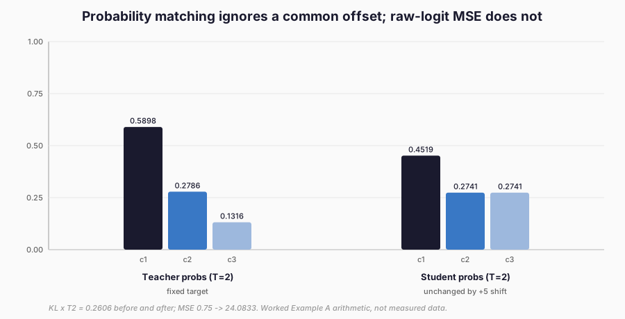
Figure 2. The same probabilities as Example A, drawn as bars, with the loss values beside them. Adding 5 to every student logit leaves every bar — and the scaled KL of 0.2606 — unchanged, while the raw-logit MSE rises from 0.75 to 24.0833. Worked-example arithmetic, not measured data.
What each signal preserves
| Signal | Typical objective | Preserves | Discards or ignores | E1 arm |
|---|---|---|---|---|
| Hard class | Cross-entropy | The teacher’s chosen class | Confidence, class similarity, non-target structure | A |
| Probability | \(T^2D_{\mathrm{KL}}\) | Relative class probabilities at \(T\) | Absolute logit offset | B, C, B-T1, B-T4, B-W25, B-W75 |
| Raw logits | Class-mean MSE | Absolute logit values and offsets | Common-offset invariance; probabilities are not the direct target | D |
| Standardised logits | MSE on centred/scaled logits | Logit shape after removing offset and scale | Absolute offset and scale | Not run |
| Ranking or margin | Ranking or pairwise loss | Order or selected differences | A unique probability distribution | Not run |
| Decoupled terms | \(\alpha\)TCKD \(+\beta\)NCKD | Target/rest confidence and conditional non-target structure | The classical coupling between them | Not run |
The table separates the signal from the training objective. A hard class can be used with a soft objective, and a probability vector can be used with an MSE objective. The rows describe the common pairing, not a rule that the signal determines the loss.
The table also makes the E1 coverage visible. E1 tested probability matching and one raw-logit MSE configuration. It did not test standardised logits, ranking losses, or DKD. Those absences are not evidence of failure. They are unmeasured method variants.
When KL and logit MSE relate
There is a real mathematical relation between temperature-scaled KL and logit MSE, but it is narrower than the informal claim that the two losses are equivalent.
Let
This distinction matters. Raw-logit MSE includes the mean offset:
There are four different claims that should not be conflated:
- Exact equality of objectives. False in general.
- Equality of minimisers under a constraint. If both teacher and student logits are constrained to zero mean, the offset term vanishes. The objectives still differ by the \(1/2\) factor and by finite-temperature terms.
- Local or asymptotic approximation. The high-temperature limit is an asymptotic statement under stated assumptions.
- Similar training behaviour in an experiment. This is an empirical observation, not an identity.
E1 is relevant to the fourth category only. The logit-MSE arm did not match the KL arm’s accuracy or cross-entropy. That does not prove that logit matching is universally worse; it shows that one raw-logit configuration, with a fixed weight and no temperature, behaved worse on one synthetic task.
Standardised logits and margins
A standardised-logit objective removes the offset and scale before matching. One definition is
Centring removes a common additive offset. Positive scaling removes a common positive scale. The transformation therefore compares the shape of the logit vector rather than its absolute values. That can be useful when the teacher and student have different calibration or temperature-like scales. It also discards information: a student can match the standardised shape while producing different probabilities, and a teacher’s absolute confidence is no longer part of the target.
The gradient flows through both the centring and the scaling. That is a feature, not an implementation detail: if the transformation were detached, the student would be rewarded for matching a representation it could not influence. The stabilising \(\epsilon\) prevents division by zero when all logits are equal. For a constant vector, the centred logits are zero and the standardised output is zero.
Standardisation is not temperature scaling. Temperature divides logits before softmax and changes the probability distribution. Standardisation transforms the logits before an MSE and does not define a probability distribution at all. The two operations can be combined, but they are not interchangeable.
Ranking and margin losses take a different route. A ranking loss preserves the order of the teacher’s scores; a margin loss preserves selected differences. Ranking information alone does not determine a unique probability distribution: many distributions share the same ordering. A margin objective preserves more than an ordering but less than the full vector. These methods are useful when the application cares about relative preference rather than calibrated probabilities. They are not a substitute for probability matching when the full distribution is the target.
The chapter does not implement a ranking loss. The contract lists it as a variant; the tested implementation covers probability matching, raw-logit MSE, standardised-logit MSE, and DKD. Adding an untested ranking objective would create the appearance of coverage without the evidence.
Decoupled knowledge distillation
The classical KL objective couples two kinds of information. It compares the teacher’s confidence on the true class with the student’s, and it compares the relative probabilities among the non-target classes. Zhao et al. (2022) show that these two parts can be separated.
Let \(t\) be the true class. Define the binary target/rest distribution
Zhao et al. introduce two weights:
The binary case needs care. If \(K=2\), there is only one non-target class, so the conditional non-target distribution is degenerate and NCKD is zero. DKD then reduces to \(\alpha\)TCKD. The implementation returns zero for NCKD in that case, and the test records the behaviour. For \(K<2\) the decomposition is not defined.
Example C. Use the same three-class pair as Example A, with target class \(t=0\) and \(T=2\).
| Quantity | Value |
|---|---|
| Teacher \(p_{T,0}^{(2)}\) | 0.5898 |
| Teacher non-target mass \(1-p_{T,0}^{(2)}\) | 0.4102 |
| Binary teacher distribution \(b_T\) | (0.5898, 0.4102) |
| Binary student distribution \(b_S\) | (0.4519, 0.5481) |
| TCKD | 0.0382 |
| Conditional teacher \(q_T\) | (0.6792, 0.3208) |
| Conditional student \(q_S\) | (0.5, 0.5) |
| NCKD | 0.0657 |
| \(T^2(\mathrm{TCKD}+(1-p_{T,0})\mathrm{NCKD})\) | 0.2606 |
| \(T^2D_{\mathrm{KL}}\) | 0.2606 |
| DKD with \(\alpha=1,\beta=2\) | 0.6781 |
The reconstructed value matches the direct KL. That is the check that matters: the decomposition is not a new approximation, it is an identity. The DKD value with \(\beta=2\) is larger because it deliberately gives NCKD more weight than the classical objective does.
The implementation exposes the terms separately:
from examples.classical_distillation.dkd import dkd_loss, dkd_terms

terms = dkd_terms(teacher_logits, student_logits, targets, temperature=2.0)
loss = dkd_loss(
    teacher_logits,
    student_logits,
    targets,
    temperature=2.0,
    alpha=1.0,
    beta=2.0,
)
dkd_terms returns per-example TCKD, NCKD, and the teacher’s target
probability. vanilla_kl_from_terms reconstructs the classical scaled KL for
testing. dkd_loss applies the separate weights. The tests check the
three-class values, the binary case, invalid targets and temperatures, and the
teacher-isolation boundary.
The DKD paper reports gains on CIFAR-100 and ImageNet. Those results are established background from that paper, not a measurement by this repository. The decomposition and equations above were checked against the arXiv v2 full text (retrieved 13 November 2026); the reported experiments were not rerun. E1 did not run DKD, standardised logits, or a ranking loss. No claim about their performance on E1 is made here.
Choosing a signal
A method-selection decision should start with access and compatibility, not with the loss’s reputation. If the teacher exposes only hard labels, probability matching is unavailable. If the teacher and student use different tokenisers or output spaces, neither raw-logit matching nor probability matching is meaningful until the spaces are aligned. Chapter 03 treats those constraints; this chapter assumes a shared classifier output space.
The second question is which invariance the application needs. If a common offset in the teacher’s logits is an artefact of the teacher’s parameterisation, probability matching or standardised logits are the safer choice. If absolute scores carry useful information, raw-logit MSE may be appropriate, but the objective should say so. If only relative order matters, a ranking or margin loss may be enough; it should not be described as full distribution matching.
The third question is what the evaluation can support. A validation split can choose a temperature or weight. The held-out test set is used once to report the result. A small sweep on one synthetic task does not establish a general ranking, and a paper’s reported gain on a different dataset is background, not a replication. The simplest defensible default is the hard-label baseline plus a probability-matching arm. Add logit or decoupled objectives when the access regime and the evaluation justify the extra assumptions.
The E1 arm matrix
E1 already contains the comparison this chapter needs. The primary group is
E1-20261112T233716Z-3bdf03, protocol 1.1, with three seeds. All arms share the
same student architecture (228 parameters), optimiser, batch size, maximum
epochs, and per-seed partitions. They do not all share the same validation
objective, and all student runs reached the 150-epoch cap. Those limits are part
of the result.
The complete arm table is:
| Arm | Supervision | Accuracy (%) | CE | ECE | Agreement (%) |
|---|---|---|---|---|---|
| A | Hard labels | 66.87 ± 3.62 | 0.8733 ± 0.0663 | 0.1461 ± 0.0189 | 66.97 ± 3.63 |
| B | Mixed KL, \(T=2\), \(\lambda=0.5\) | 64.20 ± 1.71 | 0.8651 ± 0.0258 | 0.0894 ± 0.0187 | 64.30 ± 1.75 |
| C | KL only, \(T=2\) | 62.93 ± 3.35 | 0.8578 ± 0.0880 | 0.0675 ± 0.0199 | 63.03 ± 3.36 |
| D | CE + \(0.5\) raw-logit MSE | 57.90 ± 8.94 | 0.8990 ± 0.1755 | 0.1117 ± 0.0290 | 58.00 ± 8.91 |
| B-T1 | Mixed KL, \(T=1\), \(\lambda=0.5\) | 63.00 ± 2.43 | 0.9197 ± 0.0658 | 0.1339 ± 0.0166 | 63.07 ± 2.32 |
| B-T4 | Mixed KL, \(T=4\), \(\lambda=0.5\) | 59.17 ± 8.34 | 0.9594 ± 0.1059 | 0.0771 ± 0.0207 | 59.27 ± 8.33 |
| B-W25 | Mixed KL, \(T=2\), \(\lambda=0.25\) | 65.07 ± 6.00 | 0.8391 ± 0.0849 | 0.1073 ± 0.0220 | 65.17 ± 5.90 |
| B-W75 | Mixed KL, \(T=2\), \(\lambda=0.75\) | 62.33 ± 1.15 | 0.8555 ± 0.0100 | 0.0668 ± 0.0153 | 62.43 ± 1.24 |
The standard deviations are across three seeds. They describe variability in this run; they are not confidence intervals and do not support a significance claim.
Several patterns are visible, and none of them is a universal ranking.
- No output-distillation arm beat the hard-label baseline on mean accuracy.
- The KL arms had lower mean ECE than the baseline, but every one of them had lower mean accuracy, and their cross-entropy was mixed. B, C, B-W25, and B-W75 had lower mean CE than A; B-T1 and B-T4 had higher mean CE. The calibration improvement did not translate into correctness.
- The raw-logit MSE arm had the lowest mean accuracy and the largest seed spread. Its mean cross-entropy was worse than the baseline, though not the highest in the matrix. It was a combined CE plus \(0.5\) MSE objective, not a pure logit-matching arm, so it is not a clean test of logit matching by itself.
- The temperature and weight sweeps are descriptive. They were not used to pick a winner on the test set. A different temperature might have produced a different ordering without establishing a general rule.
- B-W25 came closest to the baseline on accuracy and had the lowest mean CE. B-W75 had the lowest ECE. Those are different objectives and different trade-offs, not a single “best” arm.
The cost view is separate. Every student has 228 parameters and a 912-byte state dict. Mean training time ranged from about 4.76 s to 8.32 s across arms, and median latency was in the range of roughly 0.03–0.05 ms per measured batch in this environment. Both are host-sensitive. Neither is a capability claim, and the latency differences are too small and too noisy to rank the methods.
Evaluation and rights
The comparison has to keep four questions separate:
- Correctness. Did the student classify held-out examples correctly? Accuracy and cross-entropy answer this.
- Teacher agreement. How often does the student predict the teacher’s class? This is a diagnostic, not correctness.
- Calibration. Does confidence match empirical accuracy? ECE answers this.
- Cost. Parameters, artefact size, latency, memory, and training time answer this.
A method can improve one and worsen another. E1 is an example: the KL arms improved calibration while reducing accuracy. A deployment decision has to say which property matters for the application.
The rights question is independent of the loss. Teacher probabilities and logits
are outputs. They may be subject to service terms, output-use restrictions,
confidentiality obligations, personal-data rules, and training-data permissions.
A probability vector is still data. E1 used a self-created teacher and data
under RM-101, whose authorised action is train_and_evaluate_e1; it did not
use an external teacher or redistribute a student. That permission does not
extend to unrelated training or distribution.
Whether a particular provider’s probability vector counts as “Output” under its competing-model clause remains an open interpretive question. It is not needed for E1, which used no external outputs. Chapter 07 treats restricted access and provider terms directly; Chapters 36–39 develop the legal framework. The chapter does not treat public availability as permission.
The signal is a design choice
The output signal is now a design choice rather than a default. Probability matching preserves relative class probabilities at a temperature. Raw-logit MSE preserves absolute scores and penalises offsets. Standardised matching preserves shape but discards scale. DKD separates target confidence from non-target structure. None of these choices is universally superior.
The E1 result remains the anchor. A student can have lower cross-entropy and better calibration and still be less accurate than a hard-label baseline. The objective defines what is optimised. Held-out evaluation decides whether the result is useful.
Limits of this chapter’s evidence
- Set-up: the arm matrix comes from one synthetic task with one small teacher–student pair.
- Measurements: the ± values are standard deviations across three seeds, not confidence intervals, and they do not support a significance claim. Training time and latency are host-sensitive and do not rank the methods.
- Implementation: the arms did not all share a validation objective, and every student run reached the 150-epoch cap. Arm D combined cross-entropy with \(0.5\) raw-logit MSE at one setting, so it is not a clean test of logit matching. The temperature and weight sweeps are descriptive.
- Scope: standardised logits, ranking losses, and DKD were not run on E1. The DKD gains on CIFAR-100 and ImageNet are reported by its authors and were not rerun here. Examples A and C are worked arithmetic, not measurements.
What comes next
Chapter 07 keeps the same question but removes the full-output assumption. If the teacher exposes only top-1 labels, top-k probabilities, or sampled text, the student no longer receives the full distribution. The next chapter treats that restriction as part of the method: query cost, coverage, truncation bias, caching, and the provider terms that govern output use.
References
Ba, J. and Caruana, R. (2014). Do Deep Nets Really Need to be Deep? Advances in Neural Information Processing Systems. arXiv:1312.6184. https://arxiv.org/abs/1312.6184
Hinton, G., Vinyals, O. and Dean, J. (2015). Distilling the Knowledge in a Neural Network. NIPS 2014 Deep Learning Workshop. arXiv:1503.02531. https://arxiv.org/abs/1503.02531
Zhao, B., Cui, Q., Song, R., Qiu, Y. and Liang, J. (2022). Decoupled Knowledge Distillation. Proceedings of the IEEE/CVF Conference on Computer Vision and Pattern Recognition (CVPR), pp. 11953–11962. arXiv:2203.08679. https://arxiv.org/abs/2203.08679